Deep Learning of Vortex Induced Vibrations

Vortex induced vibrations of bluff bodies occur when the vortex shedding frequency is close to the natural frequency of the structure. Of interest is the prediction of the lift and drag forces on the structure given some limited and scattered information on the velocity field. This is an inverse problem that is not straightforward to solve using standard computational fluid dynamics (CFD) methods, especially since no information is provided for the pressure. An even greater challenge is to infer the lift and drag forces given some dye or smoke visualizations of the flow field. Here we employ deep neural networks that are extended to encode the incompressible Navier-Stokes equations coupled with the structure’s dynamic motion equation. In the first case, given scattered data in space-time on the velocity field and the structure’s motion, we use four coupled deep neural networks to infer very accurately the structural parameters, the entire time-dependent pressure field (with no prior training data), and reconstruct the velocity vector field and the structure’s dynamic motion. In the second case, given scattered data in space-time on a concentration field only, we use five coupled deep neural networks to infer very accurately the vector velocity field and all other quantities of interest as before. This new paradigm of inference in fluid mechanics for coupled multi-physics problems enables velocity and pressure quantification from flow snapshots in small subdomains and can be exploited for flow control applications and also for system identification.

Problem Setup and Solution Methodology

We begin by considering the prototype Vortex induced vibrations VIV problem of flow past a circular cylinder. The fluid motion is governed by the incompressible Navier-Stokes equations while the dynamics of the structure is described in a general form involving displacement, velocity, and acceleration terms. In particular, let us consider the two-dimensional version of flow over a flexible cable, i.e., an elastically mounted cylinder. The two-dimensional problem contains most of the salient features of the three-dimensional case and consequently it is relatively straightforward to generalize the proposed framework to the flexible cylinder/cable problem. In two dimensions, the physical model of the cable reduces to a mass-spring-damper system. There are two directions of motion for the cylinder: the streamwise (i.e., \(x\)) direction and the crossflow (i.e., \(y\)) direction. In this work, we assume that the cylinder can only move in the crossflow (i.e., \(y\)) direction; we concentrate on crossflow vibrations since this is the primary VIV direction. However, it is a simple extension to study cases where the cylinder is free to move in both streamwise and crossflow directions.

A Pedagogical Example

The cylinder displacement is defined by the variable \(\eta\) corresponding to the crossflow motion. The equation of motion for the cylinder is then given by

where \(\rho\), \(b\), and \(k\) are the mass, damping, and stiffness parameters, respectively. The fluid lift force on the structure is denoted by \(f_L\). The mass \(\rho\) of the cylinder is usually a known quantity; however, the damping \(b\) and the stiffness \(k\) parameters are often unknown in practice. In the current work, we put forth a deep learning approach for estimating these parameters from measurements. We start by assuming that we have access to the input-output data \(\{t^n, \eta^n\}_{n=1}^N\) and \(\{t^n, f_L^n\}_{n=1}^N\) on the displacement \(\eta(t)\) and the lift force \(f_L(t)\) functions, respectively. Having access to direct measurements of the forces exerted by the fluid on the structure is obviously a strong assumption. However, we start with this simpler but pedagogical case and we will relax this assumption later in this section.

Inspired by recent developments in physics informed deep learning and deep hidden physics models, we propose to approximate the unknown function \(\eta\) by a deep neural network. This choice is motivated by modern techniques for solving forward and inverse problems involving partial differential equations, where the unknown solution is approximated either by a neural network or a Gaussian process. Moreover, placing a prior on the solution is fully justified by similar approaches pursued in the past centuries by classical methods of solving partial differential equations such as finite elements, finite differences, or spectral methods, where one would expand the unknown solution in terms of an appropriate set of basis functions. Approximating the unknown function \(\eta\) by a deep neural network and using the above equation allow us to obtain the following physics-informed neural network (see the following figure)

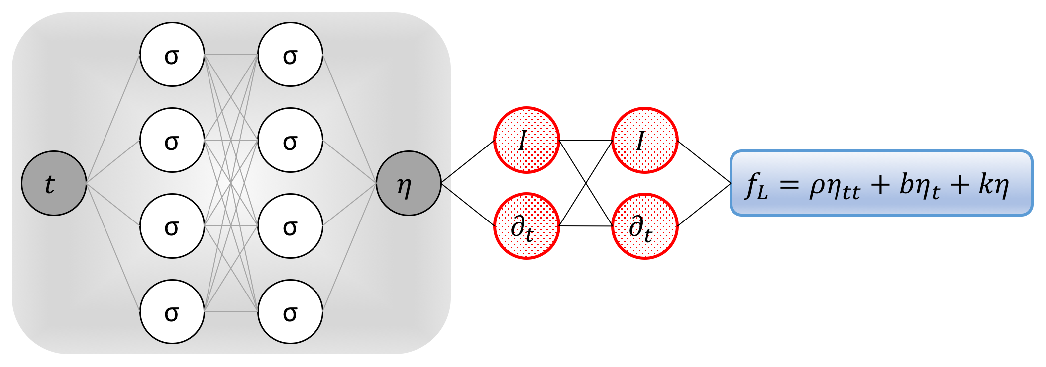
It is worth noting that the damping \(b\) and the stiffness \(k\) parameters turn into parameters of the resulting physics informed neural network \(f_L\). We obtain the required derivatives to compute the residual network \(f_L\) by applying the chain rule for differentiating compositions of functions using automatic differentiation. Automatic differentiation is different from, and in several respects superior to, numerical or symbolic differentiation – two commonly encountered techniques of computing derivatives. In its most basic description, automatic differentiation relies on the fact that all numerical computations are ultimately compositions of a finite set of elementary operations for which derivatives are known. Combining the derivatives of the constituent operations through the chain rule gives the derivative of the overall composition. This allows accurate evaluation of derivatives at machine precision with ideal asymptotic efficiency and only a small constant factor of overhead. In particular, to compute the required derivatives we rely on Tensorflow, which is a popular and relatively well documented open source software library for automatic differentiation and deep learning computations.

The shared parameters of the neural networks \(\eta\) and \(f_L\), in addition to the damping \(b\) and the stiffness \(k\) parameters, can be learned by minimizing the following sum of squared errors loss function

The first summation in this loss function corresponds to the training data on the displacement \(\eta(t)\) while the second summation enforces the dynamics imposed by equation of motion for the cylinder.

Inferring Lift and Drag Forces from Scattered Velocity Measurements

So far, we have been operating under the assumption that we have access to direct measurements of the lift force \(f_L\). In the following, we are going to relax this assumption by recalling that the fluid motion is governed by the incompressible Navier-Stokes equations given explicitly by

Here, \(u(t,x,y)\) and \(v(t,x,y)\) are the streamwise and crossflow components of the velocity field, respectively, while \(p(t,x,y)\) denotes the pressure, and \(Re\) is the Reynolds number based on the cylinder diameter and the free stream velocity. We consider the incompressible Navier-Stokes equations in the coordinate system attached to the cylinder, so that the cylinder appears stationary in time. This explains the appearance of the extra term \(\eta_{tt}\) in the second momentum equation.

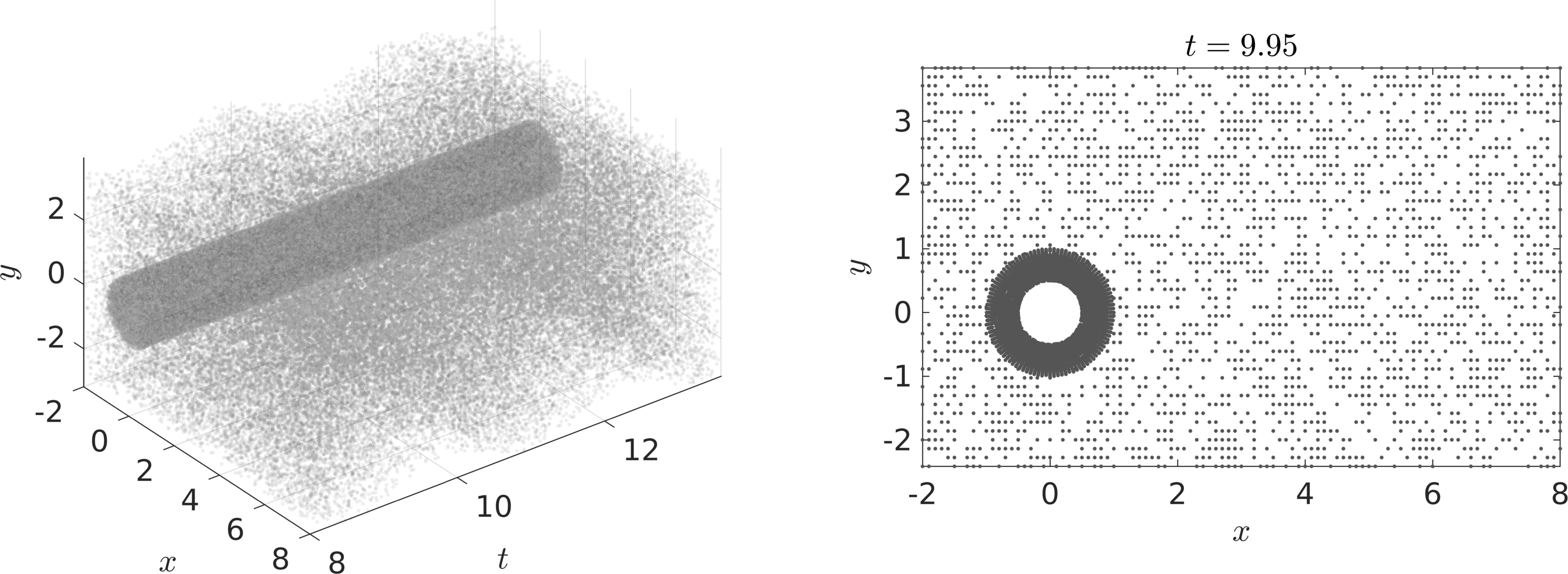
Problem 1 (VIV-I): Given scattered and potentially noisy measurements \(\{t^n, x^n, y^n, u^n, v^n\}_{n=1}^N\) of the velocity field – Take for example the case of reconstructing a flow field from scattered measurements obtained from Particle Image Velocimetry (PIV) or Particle Tracking Velocimetry (PTV) – in addition to the data \(\{t^n,\eta^n\}_{n=1}^{N}\) on the displacement and knowing the governing equations of the flow, we are interested in reconstructing the entire velocity field as well as the pressure field in space-time. Such measurements are usually collected only in a small sub-domain, which may not be appropriate for classical CFD computations due to the presence of numerical artifacts. Typically, the data points are scattered in both space and time and are usually of the order of a few thousands or less in space. For a visual representation of the distribution of observation points \(\{t^n, x^n, y^n\}_{n=1}^N\) scattered in space and time please refer to the following figure.

To solve the aforementioned problem, we proceed by approximating the latent functions \(u(t,x,y)\), \(v(t,x,y)\), \(p(t,x,y)\), and \(\eta(t)\) by a single neural network outputting four variables while taking as input \(t, x\), and \(y\). This prior assumption along with the incompressible Navier-Stokes equations result in the following Navier-Stokes informed neural networks (see the following figure)

We use automatic differentiation to obtain the required derivatives to compute the residual networks \(e_1\), \(e_2\), and \(e_3\). The shared parameters of the neural networks \(u\), \(v\), \(p\), \(\eta\), \(e_1\), \(e_2\), and \(e_3\) can be learned by minimizing the sum of squared errors loss function

Here, the first two summations correspond to the training data on the fluid velocity and the structure displacement while the last summation enforces the dynamics imposed by the incompresible Navier-Stokes equations.

The fluid forces on the cylinder are functions of the pressure and the velocity gradients. Consequently, having trained the neural networks, we can use

to obtain the lift and drag forces exerted by the fluid on the cylinder. Here, \((n_x,n_y)\) is the outward normal on the cylinder and \(ds\) is the arc length on the surface of the cylinder. We use the trapezoidal rule to approximately compute these integrals, and we use the above equations to obtain the required data on the lift force. These data are then used to estimate the structural parameters \(b\) and \(k\) by minimizing the first loss function introduced in this document.

Inferring Lift and Drag Forces from Flow Visualizations

We now consider the second VIV learning problem by taking one step further and circumvent the need for having access to measurements of the velocity field by leveraging the following equation

governing the evolution of the concentration \(c(t,x,y)\) of a passive scalar injected into the fluid flow dynamics described by the incompressible Navier-Stokes equations. Here, \(Pe\) denotes the Péclet number, defined based on the cylinder diameter, the free-stream velocity and the diffusivity of the concentration species.

Problem 2 (VIV-II): Given scattered and potentially noisy measurements \(\{t^n,x^n,y^n,c^n\}_{n=1}^N\) of the concentration \(c(t,x,y)\) of the passive scalar in space-time, we are interested in inferring the latent (hidden) quantities \(u(t,x,y)\), \(v(t,x,y)\), and \(p(t,x,y)\) while leveraging the governing equations of the flow as well as the transport equation describing the evolution of the passive scalar. Typically, the data points are of the order of a few thousands or less in space. Moreover, the equations for lift and drag enable us to consequently compute the drag and lift forces, respectively, as functions of the inferred pressure and velocity gradients. Unlike the first VIV problem, here we assume that we do not have access to direct observations of the velocity field.

To solve the second VIV problem, in addition to approximating \(u(t,x,y)\), \(v(t,x,y)\), \(p(t,x,y)\), and \(\eta(t)\) by deep neural networks as before, we represent \(c(t,x,y)\) by yet another output of the network taking \(t, x,\) and \(y\) as inputs. This prior assumption along with the scalar transport equation result in the following additional component of the Navier-Stokes informed neural network (see the following figure)

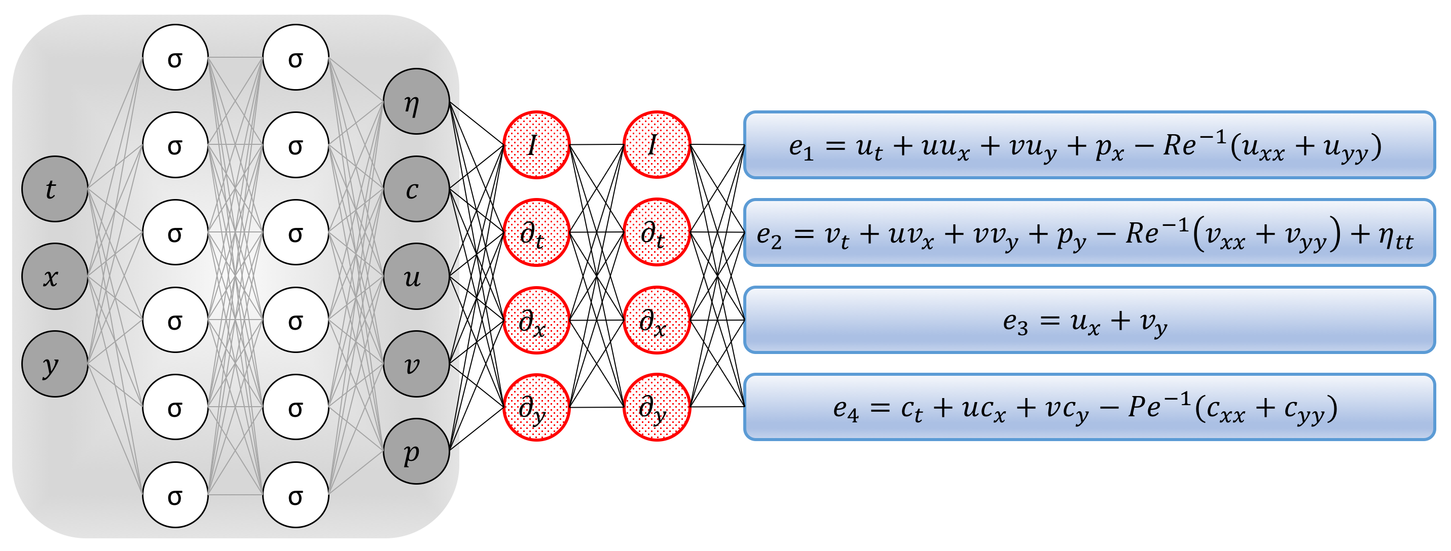
The residual networks \(e_1\), \(e_2\), and \(e_3\) are defined as before. We use automatic differentiation to obtain the required derivatives to compute the additional residual network \(e_4\). The shared parameters of the neural networks \(c\), \(u\), \(v\), \(p\), \(\eta\), \(e_1\), \(e_2\), \(e_3\), and \(e_4\) can be learned by minimizing the sum of squared errors loss function

Here, the first summation corresponds to the training data on the concentration of the passive scalar and the structure’s displacement, the second summation corresponds to the Dirichlet boundary data on the velocity field, and the last summation enforces the dynamics imposed by Navier-Stokes equations and the equation corresponding to the passive scalar. Upon training, we use the lift and drag equations to obtain the required data on the lift force. Such data are then used to estimate the structural parameters \(b\) and \(k\) by minimizing the first loss function introduced in this document.

Results

To generate a high-resolution dataset for the VIV problem we have performed direct numerical simulations (DNS) employing the high-order spectral-element method, together with the coordinate transformation method to take account of the boundary deformation. The computational domain is \([-6.5\,D,23.5\,D] \times [-10\,D,10 \, D]\), consisting of 1,872 quadrilateral elements. The cylinder center was placed at \((0, 0)\). On the inflow, located at \(x/D=-6.5\), we prescribe \((u=U_{\infty},v=0)\). On the outflow, where \(x/D=23.5\), zero-pressure boundary condition \((p=0)\) is imposed. On both top and bottom boundaries where \(y/D=\pm 10\), a periodic boundary condition is used. The Reynolds number is \(Re=100\), \(\rho=2\), \(b=0.084\) and \(k=2.2020\). For the case with dye, we assumed the Péclet number \(Pe=90\). First, the simulation is carried out until \(t=1000 \, \frac{D}{U_{\infty}}\) when the system is in steady periodic state. Then, an additional simulation for \(\Delta t=14 \,\frac{D}{U_{\infty}}\) is performed to collect the data that are saved in 280 field snapshots. The time interval between two consecutive snapshots is \(\Delta t= 0.05 \frac{D}{U_{\infty}}\). Note here \(D=1\) is the diameter of the cylinder and \(U_{\infty}=1\) is the inflow velocity. We use the DNS results to compute the lift and drag forces exerted by the fluid on the cylinder. All data and codes used in this manuscript will be publicly available on GitHub.

A Pedagogical Example

To illustrate the effectiveness of our approach, let us start with the two time series depicted in the following figure consisting of \(N=111\) observations of the displacement and the lift force. These data correspond to damping and stiffness parameters with exact values \(b=0.084\) and \(k=2.2020\), respectively. Here, the cylinder is assumed to have a mass of \(\rho = 2.0\). This data-set is then used to train a 10-layer deep neural network with 32 neurons per hidden layers by minimizing the sum of squared errors loss function (the first loss function introduced in the current work) using the Adam optimizer. Upon training, the network is used to predict the entire solution functions \(\eta(t)\) and \(f_L(t)\), as well as the unknown structural parameters \(b\) and \(k\). In addition to almost perfect reconstructions of the two time series for displacement and lift force, the proposed framework is capable of identifying the correct values for the structural parameters \(b\) and \(k\) with remarkable accuracy. The learned values for the damping and stiffness parameters are \(b = 0.08438281\) and \(k = 2.2015007\). This corresponds to around \(0.45\%\) and \(0.02\%\) relative errors in the estimated values for \(b\) and \(k\), respectively.

As for the activation functions, we use \(\sin(x)\). In general, the choice of a neural network’s architecture (e.g., number of layers/neurons and form of activation functions) is crucial and in many cases still remains an art that relies on one’s ability to balance the trade off between expressivity and trainability of the neural network. Our empirical findings so far indicate that deeper and wider networks are usually more expressive (i.e., they can capture a larger class of functions) but are often more costly to train (i.e., a feed-forward evaluation of the neural network takes more time and the optimizer requires more iterations to converge). Moreover, the sinusoid (i.e., \(\sin(x)\)) activation function seems to be numerically more stable than \(\tanh(x)\), at least while computing the residual neural networks \(f_L\), and \(e_i\), \(i=1,\ldots,4\). In this work, we have tried to choose the neural networks’ architectures in a consistent fashion throughout the manuscript by setting the number of layers to 10 and the number of neurons to 32 per output variable. Consequently, there might exist other architectures that improve some of the results reported in the current work.

Inferring Lift and Drag Forces from Scattered Velocity Measurements

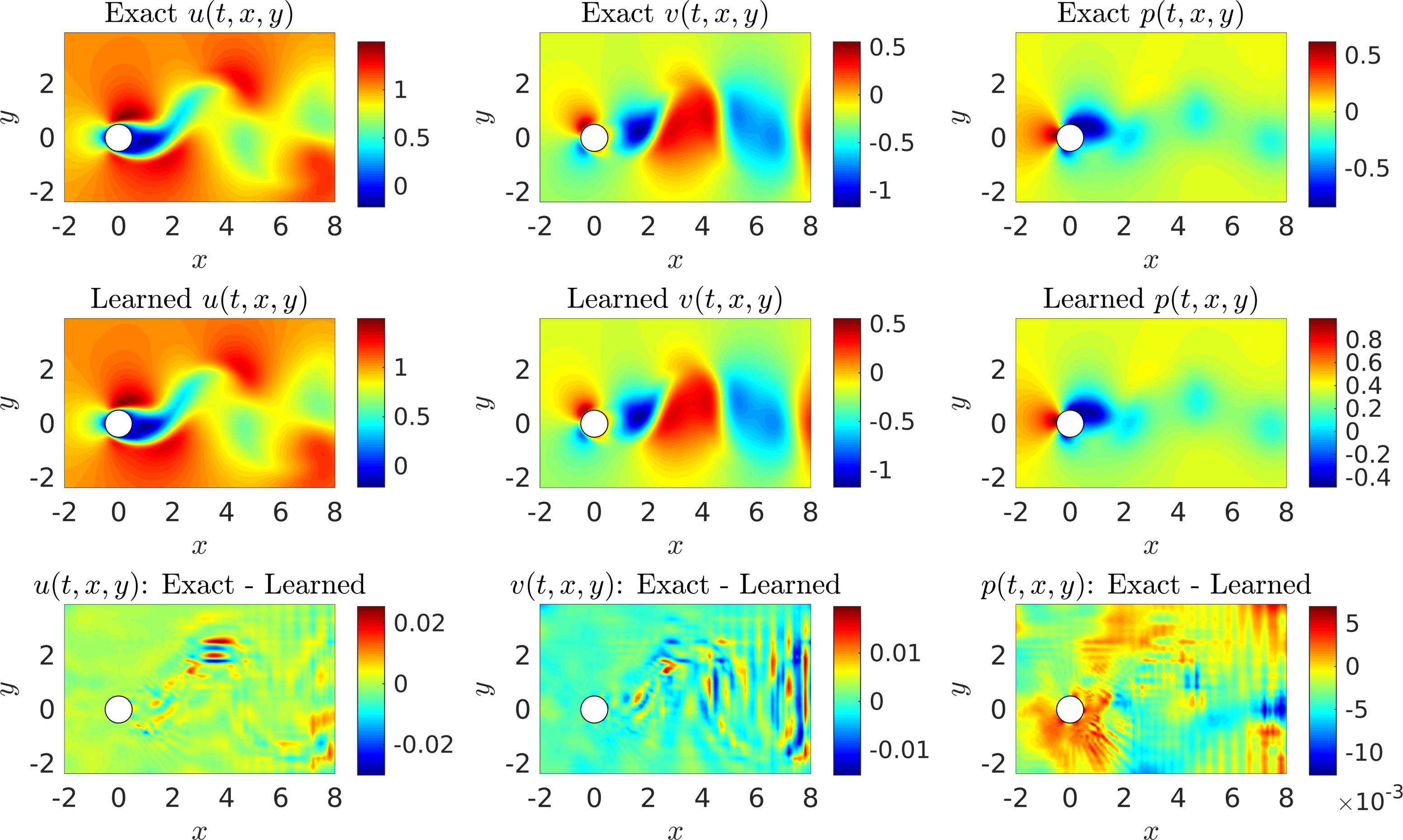
Let us now consider the case where we do not have access to direct measurements of the lift force \(f_L\). In this case, we can use measurements of the velocity field, obtained for instance via Particle Image Velocimetry (PIV) or Particle Tracking Velocimetry (PTV), to reconstruct the velocity field, the pressure, and consequently the drag and lift forces. A representative snapshot of the data on the velocity field is depicted in the top left and top middle panels of the following figure. The neural network architectures used here consist of 10 layers with 32 neurons in each hidden layer. A summary of our results is presented in the following figure. The proposed framework is capable of accurately (of the order of \(10^{-3}\)) reconstructing the velocity field; however, a more intriguing result stems from the network’s ability to provide an accurate prediction of the entire pressure field \(p(t,x,y)\) in the absence of any training data on the pressure itself (see the following figure). A visual comparison against the exact pressure is presented in the following figure for a representative snapshot of the pressure. It is worth noticing that the difference in magnitude between the exact and the predicted pressure is justified by the very nature of incompressible Navier-Stokes equations, since the pressure field is only identifiable up to a constant. This result of inferring a continuous quantity of interest from auxiliary measurements by leveraging the underlying physics is a great example of the enhanced capabilities that our approach has to offer, and highlights its potential in solving high-dimensional data assimilation and inverse problems.

The trained neural networks representing the velocity field and the pressure can be used to compute the drag and lift forces by employing equations for drag and lift, respectively. The resulting drag and lift forces are compared to the exact ones in the following figure. In the following, we are going to use the computed lift force to generate the required training data on \(f_L\) and estimate the structural parameters \(b\) and \(k\) by minimizing the the first loss function intoduced in the current work. Upon training, the proposed framework is capable of identifying the correct values for the structural parameters \(b\) and \(k\) with remarkable accuracy. The learned values for the damping and stiffness parameters are \(b = 0.0844064\) and \(k = 2.1938791\). This corresponds to around \(0.48\%\) and \(0.37\%\) relative errors in the estimated values for \(b\) and \(k\), respectively.

Inferring Lift and Drag Forces from Flow Visualizations

Let us continue with the case where we do not have access to direct observations of the lift force \(f_L\). This time rather than using data on the velocity field, we use measurements of the concentration of a passive scalar (e.g., dye or smoke) injected into the system. In the following, we are going to employ such data to reconstruct the velocity field, the pressure, and consequently the drag and lift forces. A representative snapshot of the data on the concentration of the passive scalar is depicted in the top left panel of the following figure. The neural networks’ architectures used here consist of 10 layers with 32 neurons per each hidden layer per output variable. A summary of our results is presented in the following figure. The proposed framework is capable of accurately (of the order of \(10^{-3}\)) reconstructing the concentration. However, a truly intriguing result stems from the network’s ability to provide accurate predictions of the entire velocity vector field as well as the pressure, in the absence of sufficient training data on the pressure and the velocity field themselves (see the following figure). A visual comparison against the exact quantities is presented in the following figure for a representative snapshot of the velocity field and the pressure. This result of inferring multiple hidden quantities of interest from auxiliary measurements by leveraging the underlying physics is a great example of the enhanced capabilities that physics-informed deep learning has to offer, and highlights its potential in solving high-dimensional data-assimilation and inverse problems.

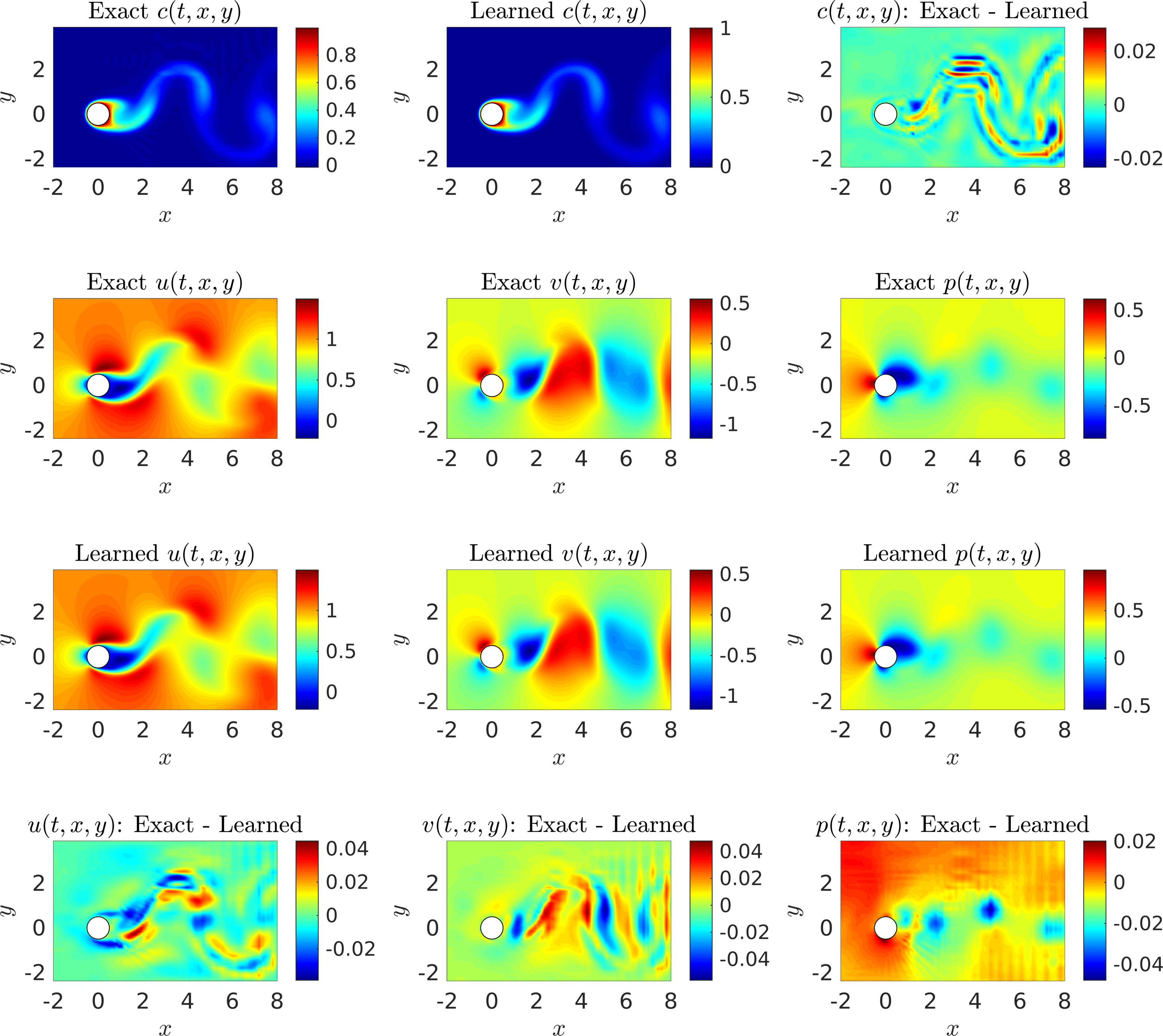
Following the same procedure as in the previous example, the trained neural networks representing the velocity field and the pressure can be used to compute the drag and lift forces by employing the equations for drag and lift, respectively. The resulting drag and lift forces are compared to the exact ones in the following figure. In the following, we are going to use the computed lift force to generate the required training data on \(f_L\) and estimate the structural parameters \(b\) and \(k\) by minimizing the first loss function introduced in the current work. Upon training, the proposed framework is capable of identifying the correct values for the structural parameters \(b\) and \(k\) with surprising accuracy. The learned values for the damping and stiffness parameters are \(b = 0.08600664\) and \(k = 2.2395933\). This corresponds to around \(2.39\%\) and \(1.71\%\) relative errors in the estimated values for \(b\) and \(k\), respectively.

Summary and Discussion

We have considered the classical coupled problem of a freely vibrating cylinder due to lift forces and demonstrated how physics informed deep learning can be used to infer quantities of interest from scattered data in space-time. In the first VIV learning problem, we inferred the pressure field and structural parameters, and hence the lift and drag on the vibrating cylinder using velocity and displacement data in time-space. In the second VIV learning problem, we inferred the velocity and pressure fields as well as the structural parameters given data on a passive scalar in space-time. The framework we propose here represents a paradigm shift in fluid mechanics simulation as it uses the governing equations as regularization mechanisms in the loss function of the corresponding minimization problem. It is particularly effective for multi-physics problems as the coupling between fields can be readily accomplished by sharing parameters among the multiple neural networks – here a neural network outputting 4 variables for the first problem and 5 variables for the second one – and for more general coupled problems by also including coupled terms in the loss function. There are many questions that this new type of modeling raises, both theoretical and practical, e.g. efficiency, solution uniqueness, accuracy, etc. We have considered such questions here in the present context as well as in our previous work in the context of physics-informed learning machines but admittedly at the present time it is not possible to rigorously answer such questions. We hope, however, that our present work will ignite interest in physics-informed deep learning that can be used effectively for many different fields of multi-physics fluid mechanics.

Moreover, it must be mentioned that we are avoiding the regimes where the Navier-Stokes equations become chaotic and turbulent (e.g., as the Reynolds number increases). In fact, it should not be difficult for a plain vanilla neural network to approximate the types of complicated functions that naturally appear in turbulence. However, as we compute the derivatives required in the computation of the physics informed neural networks, minimizing the loss functions might become a challenge, where the optimizer may fail to converge to the right values for the parameters of the neural networks. It might be the case that the resulting optimization problem inherits the complicated nature of the turbulent Navier-Stokes equations. Hence, inference of turbulent velocity and pressure fields should be considered in future extensions of this line of research. Moreover, in this work we have been operating under the assumption of Newtonian and incompressible fluid flow governed by the Navier-Stokes equations. However, the proposed algorithm can also be used when the underlying physics is non-Newtonian, compressible, or partially known. This, in fact, is one of the advantages of our algorithm in which other unknown parameters such as the Reynolds and Péclet number numbers can be inferred in addition to the velocity and pressure fields.

Acknowledgements

This work received support by the DARPA EQUiPS grant N66001-15-2-4055 and the AFOSR grant FA9550-17-1-0013. All data and codes are publicly available on GitHub.

Citation

@article{raissi2018deepVIV,
  title={Deep Learning of Vortex Induced Vibrations},
  author={Raissi, Maziar and Wang, Zhicheng and Triantafyllou, Michael S and Karniadakis, George Em},
  journal={arXiv preprint arXiv:1808.08952},
  year={2018}
}