Authors

Abstract

We introduce Hidden Physics Models, which are essentially data-efficient learning machines capable of leveraging the underlying laws of physics, expressed by time dependent and nonlinear partial differential equations, to extract patterns from high-dimensional data generated from experiments. The proposed methodology may be applied to the problem of learning, system identification, or data-driven discovery of partial differential equations. Our framework relies on Gaussian Processes, a powerful tool for probabilistic inference over functions, that enables us to strike a balance between model complexity and data fitting. The effectiveness of the proposed approach is demonstrated through a variety of canonical problems, spanning a number of scientific domains, including the Navier-Stokes, Schrödinger, Kuramoto-Sivashinsky, and time dependent linear fractional equations. The methodology provides a promising new direction for harnessing the long-standing developments of classical methods in applied mathematics and mathematical physics to design learning machines with the ability to operate in complex domains without requiring large quantities of data.

Problem Setup

Let us consider parametrized and nonlinear partial differential equations of the general form

$h_t + \mathcal{N}_x^\lambda h = 0,$

where $h(t,x)$ denotes the latent (hidden) solution and $\mathcal{N}_x^\lambda$ is a nonlinear operator parametrized by $\lambda$ . Given noisy measurements of the system, one is typically interested in the solution of two distinct problems.

The first problem is that of inference or filtering and smoothing, which states: given fixed model parameters $\lambda$ what can be said about the unknown hidden state $h(t,x)$ of the system? This question is the topic Numerical Gaussian Processes in which we address the problem of inferring solutions of time dependent and nonlinear partial differential equations using noisy observations.

The second problem is that of learning, system identification, or data driven discovery of partial differential equations stating: what are the parameters $\lambda$ that best describe the observed data?

Here, we assume that all we observe are two snapshots of the system at times $t^{n-1}$ and $t^n$ that are $\Delta t = t^n - t^{n-1}$ apart. The main assumption is that $\Delta t$ is small enough so that we can employ the backward Euler time stepping scheme and obtain the discretized equation

$h^{n} + \Delta t \mathcal{N}^\lambda_x h^n = h^{n-1}.$

Here, $h^n(x) = h(t^n,x)$ is the hidden state of the system at time $t^n$ . Approximating the nonlinear operator on the left-hand-side of this equation by a linear one we obtain

$\mathcal{L}^\lambda_x h^n = h^{n-1}.$

Prior

Similar to the ideas presented here and here, we build upon the analytical property of Gaussian processes that the output of a linear system whose input is Gaussian distributed is again Gaussian. Specifically, we proceed by placing a Gaussian process prior over the latent function $h^{n}(x)$ ; i.e.,

$h^n(x) \sim \mathcal{GP}(0, k(x,x',\theta)).$

Here, $\theta$ denotes the hyper-parameters of the covariance function $k$ . This enables us to capture the entire structure of the operator $\mathcal{L}_x^{\lambda}$ in the resulting multi-output Gaussian process

$\begin{bmatrix} h^{n} \\ h^{n-1} \end{bmatrix} \sim \mathcal{GP}\left(0, \begin{bmatrix} k^{n,n} & k^{n,n-1}\\ k^{n-1,n} & k^{n-1,n-1} \end{bmatrix} \right).$

We call the resulting multi-output Gaussian process a Hidden Physics Model, because its matrix of covariance functions explicitly encodes the underlying laws of physics expressed by the corresponding partial differential equation.

Learning

Given noisy data $\{\mathbf{x}^{n-1}, \mathbf{h}^{n-1}\}$ and $\{\mathbf{x}^{n}, \mathbf{h}^{n}\}$ on the latent solution at times $t^{n-1}$ and $t^n$ , respectively, the hyper-parameters $\theta$ of the covariance functions and more importantly the parameters $\lambda$ of the operators $\mathcal{L}_x^\lambda$ and $\mathcal{N}_x^\lambda$ can be learned by employing a Quasi-Newton optimizer L-BFGS to minimize the negative log marginal likelihood

$-\log p(\mathbf{h}| \theta, \lambda, \sigma^2) = \frac{1}{2} \mathbf{h}^{T}\mathbf{K}^{-1}\mathbf{h} + \frac{1}{2}\log |\mathbf{K}| + \frac{N}{2} \log (2\pi),$

where $\mathbf{h} = \begin{bmatrix} \mathbf{h}^n \\ \mathbf{h}^{n-1} \end{bmatrix}$ , $p(\mathbf{h} | \theta, \lambda, \sigma^2) = \mathcal{N}\left(\mathbf{0}, \mathbf{K}\right)$ , and $\mathbf{K}$ is given by

$\mathbf{K} = \begin{bmatrix} k^{n,n}(\mathbf{x}^{n},\mathbf{x}^{n}) & k^{n,n-1}(\mathbf{x}^{n},\mathbf{x}^{n-1})\\ k^{n-1,n}(\mathbf{x}^{n-1},\mathbf{x}^{n}) & k^{n-1,n-1}(\mathbf{x}^{n-1},\mathbf{x}^{n-1}) \end{bmatrix} + \sigma^2 \mathbf{I}.$

Here, $N$ is the total number of data points in $\mathbf{h}$ . Moreover, $\sigma^2$ is included to capture the noise in the data and is also learned by minimizing the negative log marginal likelihood.

Kuramoto-Sivashinsky Equation

The Kuramoto-Sivashinsky equation is a canonical model of a pattern forming system with spatio-temporal chaotic behavior. The sign of the second derivative term is such that it acts as an energy source and thus has a destabilizing effect. The nonlinear term, however, transfers energy from low to high wave numbers where the stabilizing fourth derivative term dominates.

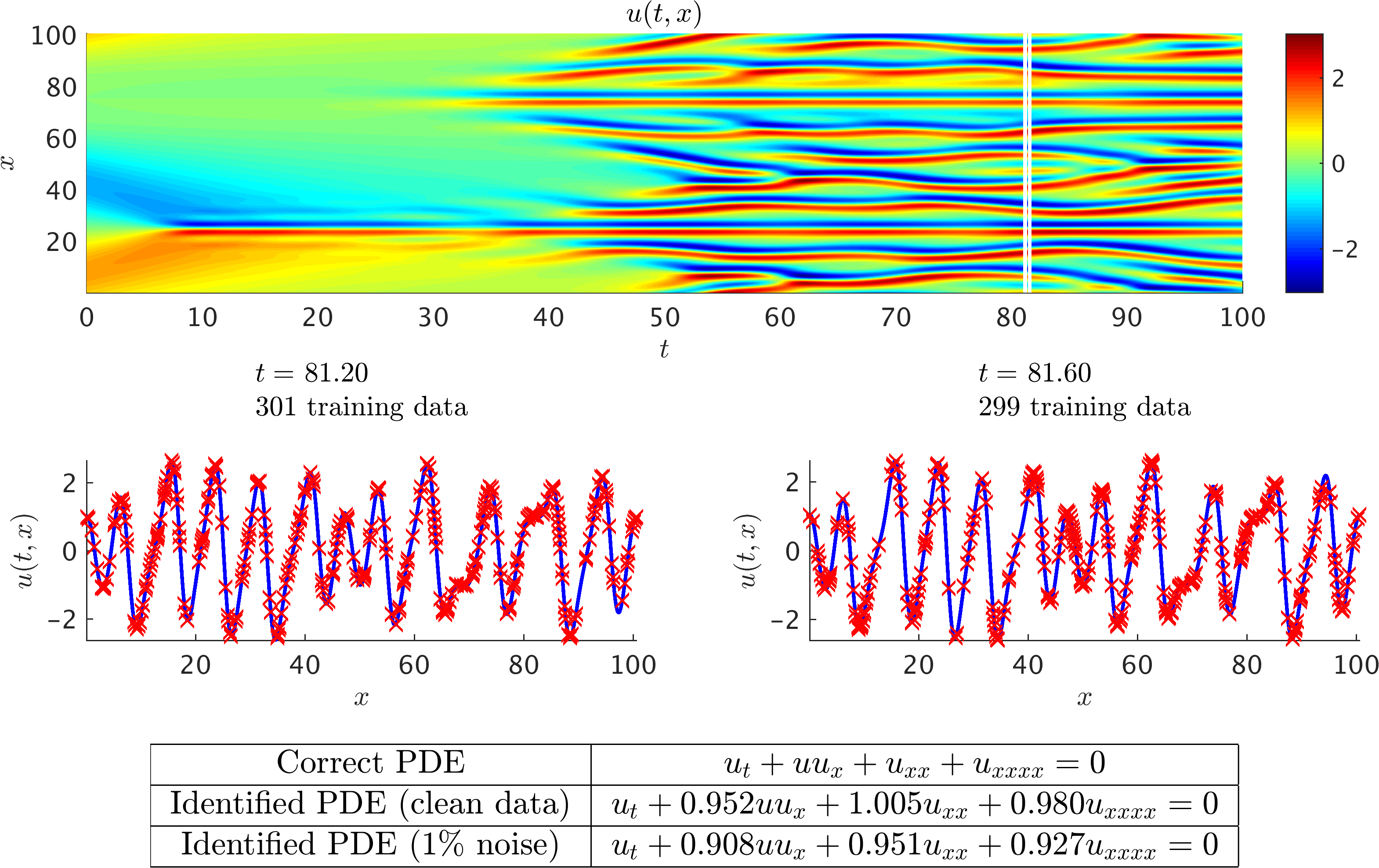
Kuramoto-Sivashinsky equation: A solution to the Kuramoto-Sivashinsky equation is depicted in the top panel. The two white vertical lines in this panel specify the locations of the two randomly selected snapshots. These two snapshots are 0.4 apart and are plotted in the middle panel. The red crosses denote the locations of the training data points. The correct partial differential equation along with the identified ones are reported in the lower panel.

Navier-Stokes Equation

Navier-Stokes equations describe the physics of many phenomena of scientific and engineering interest. They may be used to model the weather, ocean currents, water flow in a pipe and air flow around a wing. The Navier-Stokes equations in their full and simplified forms help with the design of aircraft and cars, the study of blood flow, the design of power stations, the analysis of the dispersion of pollutants, and many other applications.

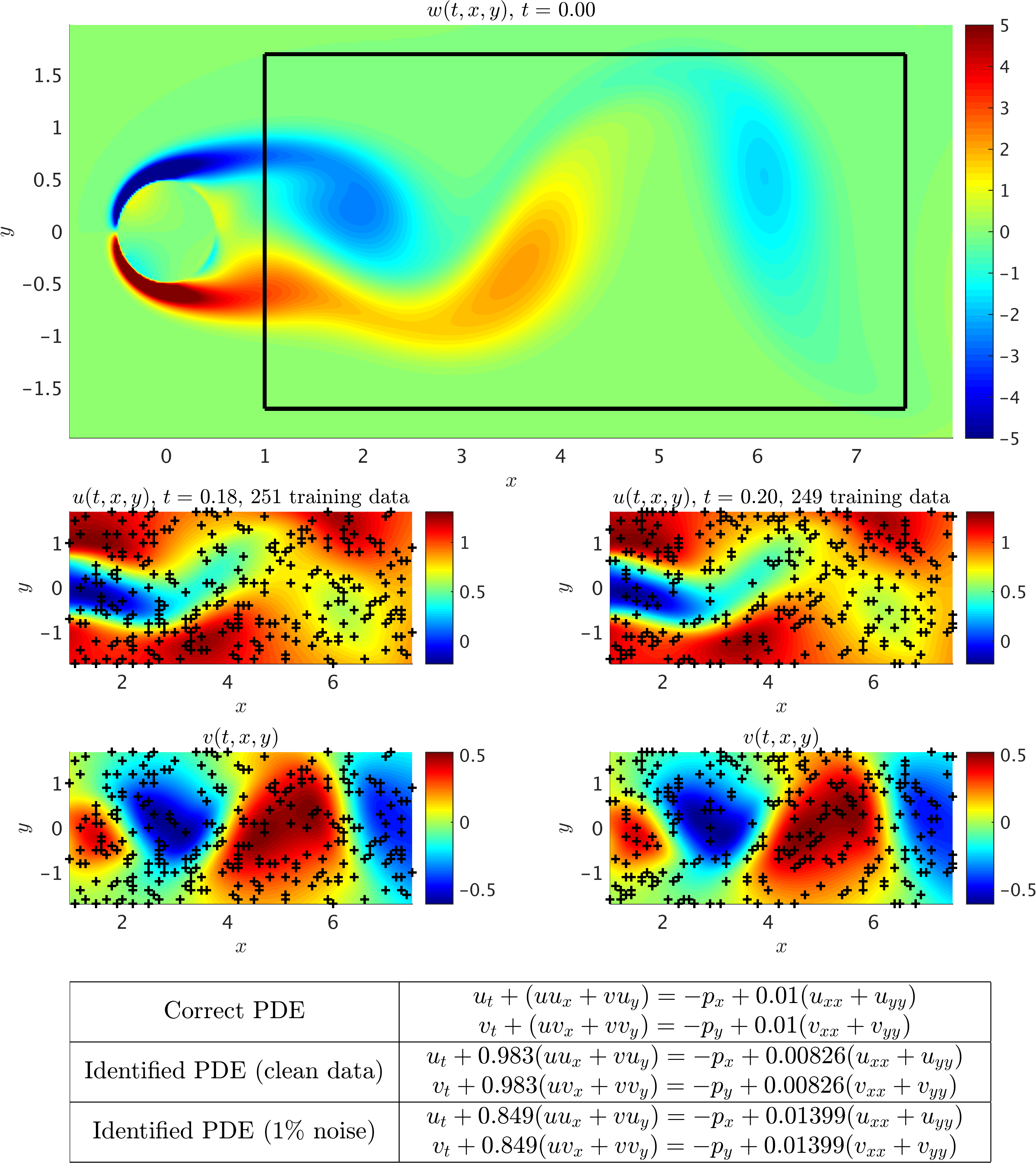
Navier-Stokes equations: A single snapshot of the vorticity field of a solution to the Navier-Stokes equations for the fluid flow past a cylinder is depicted in the top panel. The black box in this panel specifies the sampling region. Two snapshots of the velocity field being 0.02 apart are plotted in the two middle panels. The black crosses denote the locations of the training data points. The correct partial differential equation along with the identified ones are reported in the lower panel. Here, u denotes the x-component of the velocity field, v the y-component, p the pressure, and w the vorticity field.

Fractional Equations

Fractional operators often arise in modeling anomalous diffusion processes and other non-local interactions. Integer values can model classical advection and diffusion phenomena. However, under the fractional calculus setting, the fractional order can assume real values and thus continuously interpolate between inherently different model behaviors. The proposed framework allows the fractional order to be directly inferred from noisy data, and opens the path to a flexible formalism for model discovery and calibration.

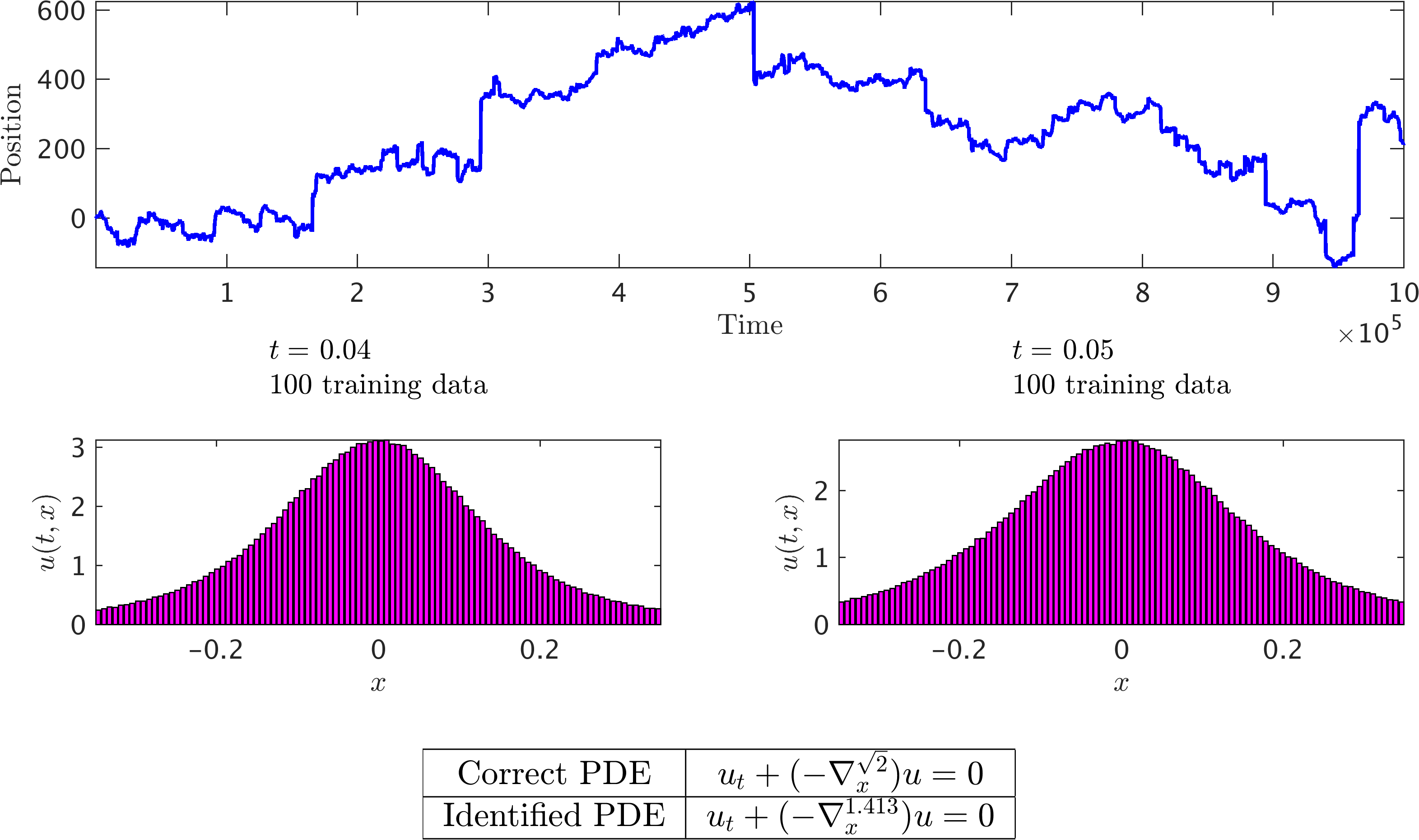
Fractional Equation – alpha-stable Levy process: A single realization of an alpha-stable Levy process is depicted in the top panel. Two histograms of the particle’s displacement, being 0.01 apart, are plotted in the middle panel. The correct partial differential equation along with the identified ones are reported in the lower panel.

Conclusion

We have introduced a structured learning machine which is explicitly informed by the underlying physics that possibly generated the observed data. Exploiting this structure is critical for constructing data-efficient learning algorithms that can effectively distill information in the data-scarce scenarios appearing routinely when we study complex physical systems. We applied the proposed framework to the problem of identifying general parametric nonlinear partial differential equations from noisy data. This generality was demonstrated using various benchmark problems with different attributes. This work should be considered a direct follow up on Numerical Gaussian Processes in which a similar methodology is employed to infer solutions to time-dependent and nonlinear partial differential equations, and effectively quantify and propagate uncertainty due to noisy initial or boundary data. The ideas introduced in these two papers provide a natural platform for learning from noisy data and computing under uncertainty.

Acknowledgements

This work received support by the DARPA EQUiPS grant N66001-15-2-4055, the MURI/ARO grant W911NF-15-1-0562, and the AFOSR grant FA9550-17-1-0013. All data and codes are publicly available on GitHub.

Citation

@article{raissi2017hidden,
  title={Hidden physics models: Machine learning of nonlinear partial differential equations},
  author={Raissi, Maziar and Karniadakis, George Em},
  journal={Journal of Computational Physics},
  year={2017},
  publisher={Elsevier}
}

Hidden Physics Models

Machine Learning of Nonlinear Partial Differential Equations

Authors

Abstract

Citation