Author

Abstract

A long-standing problem at the interface of artificial intelligence and applied mathematics is to devise an algorithm capable of achieving human level or even superhuman proficiency in transforming observed data into predictive mathematical models of the physical world. In the current era of abundance of data and advanced machine learning capabilities, the natural question arises: How can we automatically uncover the underlying laws of physics from high-dimensional data generated from experiments? In this work, we put forth a deep learning approach for discovering nonlinear partial differential equations from scattered and potentially noisy observations in space and time. Specifically, we approximate the unknown solution as well as the nonlinear dynamics by two deep neural networks. The first network acts as a prior on the unknown solution and essentially enables us to avoid numerical differentiations which are inherently ill-conditioned and unstable. The second network represents the nonlinear dynamics and helps us distill the mechanisms that govern the evolution of a given spatiotemporal data-set. We test the effectiveness of our approach for several benchmark problems spanning a number of scientific domains and demonstrate how the proposed framework can help us accurately learn the underlying dynamics and forecast future states of the system. In particular, we study the Burgers’, Korteweg-de Vries (KdV), Kuramoto-Sivashinsky, nonlinear Shrödinger, and Navier-Stokes equations.

Problem Setup

Let consider nonlinear partial differential equations of the general form

$u_t = \mathcal{N}(t,x,u,u_x,u_{xx},\ldots),$

where $\mathcal{N}$ is a nonlinear function of time $t$ , space $x$ , solution $u$ and its derivatives. Here, the subscripts denote partial differentiation in either time $t$ or space $x$ . Given a set of scattered and potentially noisy observations of the solution $u$ , we are interested in learning the nonlinear function $\mathcal{N}$ and consequently discovering the hidden laws of physics that govern the evolution of the observed data.

Solution methodology

We proceed by approximating both the solution $u$ and the nonlinear function $\mathcal{N}$ with two deep neural networks and define a deep hidden physics model $f$ to be given by

$f := u_t - \mathcal{N}(t,x,u,u_x,u_{xx},\ldots).$

We obtain the derivatives of the neural network $u$ with respect to time $t$ and space $x$ by applying the chain rule for differentiating compositions of functions using automatic differentiation. It is worth emphasizing that automatic differentiation is different from, and in several aspects superior to, numerical or symbolic differentiation; two commonly encountered techniques of computing derivatives. To compute the derivatives involved in definition above we rely on Tensorflow which is a popular and relatively well documented open source software library for automatic differentiation and deep learning computations.

Parameters of the neural networks $u$ and $\mathcal{N}$ can be learned by minimizing the sum of squared errors

$\sum_{i=1}^{N} \left(|u(t^i,x^i) - u^i|^2 + |f(t^i,x^i)|^2\right),$

where $\{t^i, x^i, u^i\}_{i=1}^{N}$ denote the training data on $u$ . The term $\mid u(t^i,x^i) - u^i\mid^2$ tries to fit the data by adjusting the parameters of the neural network $u$ while the term $\mid f(t^i,x^i)\mid^2$ learns the parameters of the network $\mathcal{N}$ by trying to satisfy the partial differential equation at the collocation points $(t^i,x^i)$ . Training the parameters of the neural networks $u$ and $\mathcal{N}$ can be performed simultaneously by minimizing the aforementioned sum of squared error or in a sequential fashion by training $u$ first and $\mathcal{N}$ second.

How can we make sure that the algorithm presented above results in an acceptable function $\mathcal{N}$ ? One answer would be to solve the learned equations and compare the resulting solution to the solution of the exact partial differential equation. However, it should be pointed out that the learned function $\mathcal{N}$ is a black-box function; i.e., we do not know its functional form. Consequently, none of the classical partial differential equation solvers such as finite differences, finite elements or spectral methods are applicable here. Therefore, to solve the learned equations we have no other choice than to resort to modern black-box solvers such as physic informed neural networks (PINNs) introduced here and here.

Results

The proposed framework provides a universal treatment of nonlinear partial differential equations of fundamentally different nature. This generality will be demonstrated by applying the algorithm to a wide range of canonical problems spanning a number of scientific domains including the Burgers’, Korteweg-de Vries (KdV), Kuramoto-Sivashinsky, nonlinear Shrödinger, and Navier-Stokes equations. All data and codes are publicly available on GitHub.

Burgers’ equation

Let us start with the Burgers’ equation arising in various areas of engineering and applied mathematics, including fluid mechanics, nonlinear acoustics, gas dynamics, and traffic flow. In one space dimension the Burgers’ equation reads as

$u_t = - u u_x + 0.1 u_{xx}.$

Given 10000 training data scatterd in space and time from time $t = 0$ to $t = 6.7$ , we are interested in learning $\mathcal{N}$ as a function of the solution $u$ and its derivatives up to the 2nd order; i.e.,

$u_t = \mathcal{N}(u,u_x,u_{xx}).$

We represent the solution $u$ by a 5-layer deep neural network with 50 neurons per hidden layer. Furthermore, we let $\mathcal{N}$ to be a neural network with 2 hidden layers and 100 neurons per hidden layer. These two networks are trained by minimizing the sum of squared errors introduced above. To illustrate the effectiveness of our approach, we solve the learned partial differential equation, along with periodic boundary conditions and the same initial condition as the one used to generate the original dataset, using the PINNs algorithm. The original dataset alongside the resulting solution of the learned partial differential equation are depicted in the following figure. This figure indicates that our algorithm is able to accurately identify the underlying partial differential equation with a relative $L^2$ -error of 4.78e-03. It should be highlighted that the training data are collected in roughly two-thirds of the domain between times $t = 0$ and $t=6.7$ . The algorithm is thus extrapolating from time $t=6.7$ onwards. The relative $L^2$ -error on the training portion of the domain is 3.89e-03.

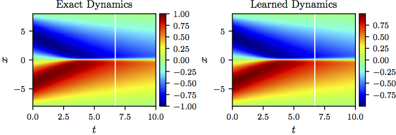
Burgers equation: A solution to the Burger’s equation (left panel) is compared to the corresponding solution of the learned partial differential equation (right panel). The identified system correctly captures the form of the dynamics and accurately reproduces the solution with a relative L2-error of 4.78e-03. It should be emphasized that the training data are collected in roughly two-thirds of the domain between times t=0 and t=6.7 represented by the white vertical lines. The algorithm is thus extrapolating from time t=6.7 onwards. The relative L2-error on the training portion of the domain is 3.89e-03.

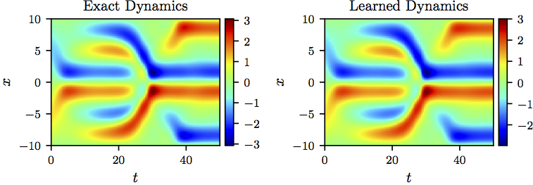
To further scrutinize the performance of our algorithm, let us change the initial condition to $-\exp(-(x+2)^2)$ and solve the Burgers’ equation using a classical partial differential equation solver. We compare the resulting solution to the one obtained by solving the learned partial differential equation using the PINNs algorithm. It is worth emphasizing that the deep hidden physics model is trained on the dataset depicted in figure above and is being tested on a totally different dataset as shown in the following figure. The surprising result reported in the following figure is a strong indication that the algorithm is capable of accurately identifying the underlying partial differential equation. The algorithm hasn’t seen even a single observation of the dataset shown in the following figure during model training and is yet capable of achieving a relatively accurate approximation of the true solution. The identified system reproduces the solution to the Burgers’ equation with a relative $L^2$ -error of 7.33e-02.

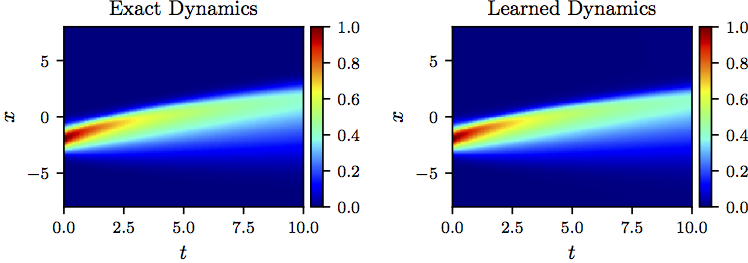
Burgers equation: A solution to the Burger’s equation (left panel) is compared to the corresponding solution of the learned partial differential equation (right panel). The identified system correctly captures the form of the dynamics and accurately reproduces the solution with a relative L2-error of 7.33e-02. It should be highlighted that the algorithm is trained on a dataset totally different from the one used in this figure.

The KdV equation

As a mathematical model of waves on shallow water surfaces one could consider the Korteweg-de Vries (KdV) equation. The KdV equation reads as

$u_t = - u u_x - u_{xxx}.$

To obtain a set of training data we simulate the KdV equation using conventional spectral methods. In particular, we start from an initial condition $u(0,x) = -\sin(\pi x/20), ~x\in [-20,20]$ and assume periodic boundary conditions. We integrate the KdV equation up to the final time $t = 40$ . Out of this dataset, we generate a smaller training subset, scattered in space and time, by randomly sub-sampling 10000 data points from time $t = 0$ to $t=26.8$ . Given the training data, we are interested in learning $\mathcal{N}$ as a function of the solution $u$ and its derivatives up to the 3rd order; i.e.,

$u_t = \mathcal{N}(u,u_x,u_{xx},u_{xxx}).$

We represent the solution $u$ by a 5-layer deep neural network with 50 neurons per hidden layer. Furthermore, we let $\mathcal{N}$ to be a neural network with 2 hidden layers and 100 neurons per hidden layer. These two networks are trained by minimizing the sum of squared errors loss discussed above. To illustrate the effectiveness of our approach, we solve the learned partial differential equation using the PINNs algorithm. We assume periodic boundary conditions and the same initial condition as the one used to generate the original dataset. The resulting solution of the learned partial differential equation as well as the exact solution of the KdV equation are depicted in the following figure. This figure indicates that our algorithm is capable of accurately identifying the underlying partial differential equation with a relative $L^2$ -error of 6.28e-02. It should be highlighted that the training data are collected in roughly two-thirds of the domain between times $t = 0$ and $t=26.8$ . The algorithm is thus extrapolating from time $t=26.8$ onwards. The corresponding relative $L^2$ -error on the training portion of the domain is 3.78e-02.

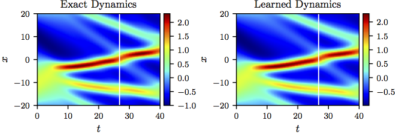
The KdV equation: A solution to the KdV equation (left panel) is compared to the corresponding solution of the learned partial differential equation (right panel). The identified system correctly captures the form of the dynamics and accurately reproduces the solution with a relative L2-error of 6.28e-02. It should be emphasized that the training data are collected in roughly two-thirds of the domain between times t = 0 and t=26.8 represented by the white vertical lines. The algorithm is thus extrapolating from time t=26.8 onwards. The relative L2-error on the training portion of the domain is 3.78e-02.

To test the algorithm even further, let us change the initial condition to $\cos(-\pi x/20)$ and solve the KdV equation using the conventional spectral method outlined above. We compare the resulting solution to the one obtained by solving the learned partial differential equation using the PINNs algorithm. It is worth emphasizing that the algorithm is trained on the dataset depicted in the figure above and is being tested on a different dataset as shown in the following figure. The surprising result reported in the following figure strongly indicates that the algorithm is accurately learning the underlying partial differential equation; i.e., the nonlinear function $\mathcal{N}$ . The algorithm hasn’t seen the dataset shown in the following figure during model training and is yet capable of achieving a relatively accurate approximation of the true solution. To be precise, the identified system reproduces the solution to the KdV equation with a relative $L^2$ -error of 3.44e-02.

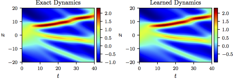
The KdV equation: A solution to the KdV equation (left panel) is compared to the corresponding solution of the learned partial differential equation (right panel). The identified system correctly captures the form of the dynamics and accurately reproduces the solution with a relative L2-error of 3.44e-02. It should be highlighted that the algorithm is trained on a dataset totally different from the one shown in this figure.

Kuramoto-Sivashinsky equation

As a canonical model of a pattern forming system with spatio-temporal chaotic behavior we consider the Kuramoto-Sivashinsky equation. In one space dimension the Kuramoto-Sivashinsky equation reads as

$u_t = - u u_x - u_{xx} - u_{xxxx}.$

We generate a dataset containing a direct numerical solution of the Kuramoto-Sivashinsky. To be precise, assuming periodic boundary conditions, we start from the initial condition $u(0,x) = -\sin(\pi x/10), ~x\in [-10,10]$ and integrate the Kuramoto-Sivashinsky equation up to the final time $t = 50$ . From this dataset, we create a smaller training subset, scattered in space and time, by randomly sub-sampling 10000 data points from time $t = 0$ to the final time $t=50.0$ . Given the resulting training data, we are interested in learning $\mathcal{N}$ as a function of the solution $u$ and its derivatives up to the 4rd order; i.e.,

$u_t = \mathcal{N}(u,u_x,u_{xx},u_{xxx},u_{xxxx}).$

We let the solution $u$ to be represented by a 5-layer deep neural network with 50 neurons per hidden layer. Furthermore, we approximate the nonlinear function $\mathcal{N}$ by a neural network with 2 hidden layers and 100 neurons per hidden layer. These two networks are trained by minimizing the sum of squared errors loss explained above. To demonstrate the effectiveness of our approach, we solve the learned partial differential equation using the PINNs algorithm. We assume the same initial and boundary conditions as the ones used to generate the original dataset. The resulting solution of the learned partial differential equation alongside the exact solution of the Kuramoto-Sivashinsky equation are depicted in the following figure. This figure indicates that our algorithm is capable of identifying the underlying partial differential equation with a relative L2-error of 7.63e-02.

Kuramoto-Sivashinsky equation: A solution to the Kuramoto-Sivashinsky equation (left panel) is compared to the corresponding solution of the learned partial differential equation (right panel). The identified system correctly captures the form of the dynamics and reproduces the solution with a relative L2-error of 7.63e-02.

Nonlinear Shrödinger equation

The one-dimensional nonlinear Shrödinger equation is a classical field equation that is used to study nonlinear wave propagation in optical fibers and/or waveguides, Bose-Einstein condensates, and plasma waves. This example aims to highlight the ability of our framework to handle complex-valued solutions as well as different types of nonlinearities in the governing partial differential equations. The nonlinear Shrödinger equation is given by

$\psi_t = 0.5 i \psi_{xx} + i |\psi|^2 \psi.$

Let $u$ denote the real part of $\psi$ and $v$ the imaginary part. Then, the nonlinear Shrödinger equation can be equivalently written as a system of partial differential equations

$\begin{array}{l} u_t = - 0.5 v_{xx} - (u^2 + v^2) v,\\ v_t = 0.5 u_{xx} + (u^2 + v^2) u. \end{array}$

In order to assess the performance of our method, we simulate the nonlinear Shrödinger equation using conventional spectral methods to create a high-resolution dataset. Specifically, starting from an initial state $\psi(0,x) = 2\ \text{sech}(x)$ and assuming periodic boundary conditions $\psi(t,-5) = \psi(t,5)$ and $\psi_x(t,-5) = \psi_x(t,5)$ , we integrate the nonlinear Shrödinger equation up to a final time $t=\pi/2$ . Out of this data-set, we generate a smaller training subset, scattered in space and time, by randomly sub-sampling 10000 data points from time $t = 0$ up to the final time $t=\pi/2$ . Given the resulting training data, we are interested in learning two nonlinear functions $\mathcal{N}_1$ and $\mathcal{N}_2$ as functions of the solutions $u, v$ and their derivatives up to the 2nd order; i.e.,

$\begin{array}{l} u_t = \mathcal{N}_1(u,v,u_x,v_x,u_{xx},v_{xx}),\\ v_t = \mathcal{N}_2(u,v,u_x,v_x,u_{xx},v_{xx}). \end{array}$

We represent the solutions $u$ and $v$ by two 5-layer deep neural networks with 50 neurons per hidden layer. Furthermore, we let $\mathcal{N}_1$ and $\mathcal{N}_2$ to be two neural networks with 2 hidden layers and 100 neurons per hidden layer. These four networks are trained by minimizing the sum of squared errors loss explained above. To illustrate the effectiveness of our approach, we solve the learned partial differential equation, along with periodic boundary conditions and the same initial condition as the one used to generate the original dataset, using the PINNs algorithm. The original dataset (in absolute values, i.e., $\vert \psi\vert = \sqrt{u^2+v^2}$ ) alongside the resulting solution (also in absolute values) of the learned partial differential equation are depicted in the following figure. This figure indicates that our algorithm is able to accurately identify the underlying partial differential equation with a relative $L^2$ -error of 6.28e-03.

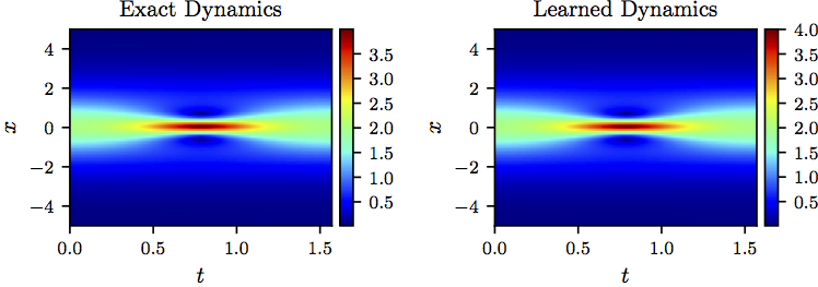
Nonlinear Shrödinger equation: Absolute value of a solution to the nonlinear Shrödinger equation (left panel) is compared to the absolute value of the corresponding solution of the learned partial differential equation (right panel). The identified system correctly captures the form of the dynamics and accurately reproduces the absolute value of the solution with a relative L2-error of 6.28e-03.

Navier-Stokes equation

Let us consider the Navier-Stokes equation in two dimensions (2D) given explicitly by

$\begin{array}{c} w_t = - u w_x - v w_y + 0.01(w_{xx} + w_{yy}), \end{array}$

where $w$ denotes the vorticity, $u$ the $x$ -component of the velocity field, and $v$ the $y$ -component. We simulate the Navier-Stokes equations describing the two-dimensional fluid flow past a circular cylinder at Reynolds number 100 using the Immersed Boundary Projection Method. This approach utilizes a multi-domain scheme with four nested domains, each successive grid being twice as large as the previous one. Length and time are nondimensionalized so that the cylinder has unit diameter and the flow has unit velocity. Data is collected on the finest domain with dimensions $9 \times 4$ at a grid resolution of $449 \times 199$ . The flow solver uses a 3rd-order Runge Kutta integration scheme with a time step of $\Delta t = 0.02$ , which has been verified to yield well-resolved and converged flow fields. After simulation converges to steady periodic vortex shedding, 151 flow snapshots are saved every $\Delta t = 0.02$ . We use a small portion of the resulting data-set for model training. In particular, we subsample 50000 data points, scattered in space and time, in the rectangular region (dashed red box) downstream of the cylinder as shown in the following figure.

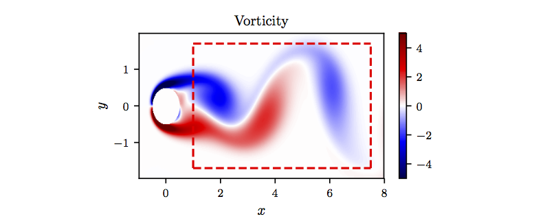
Navier-Stokes equation: A snapshot of the vorticity field of a solution to the Navier-Stokes equations for the fluid flow past a cylinder. The dashed red box in this panel specifies the sampling region.

Given the training data, we are interested in learning $\mathcal{N}$ as a function of the stream-wise $u$ and transverse $v$ velocity components in addition to the vorticity $w$ and its derivatives up to the 2nd order; i.e.,

$w_t = \mathcal{N}(u,v,w,w_x,w_{xx}).$

We represent the solution $w$ by a 5-layer deep neural network with 200 neurons per hidden layer. Furthermore, we let $\mathcal{N}$ to be a neural network with 2 hidden layers and 100 neurons per hidden layer. These two networks are trained by minimizing the sum of squared errors loss

$\sum_{i=1}^{N} \left(|w(t^i,x^i,y^i) - w^i|^2 + |f(t^i,x^i,y^i)|^2\right),$

where $\{t^i, x^i, u^i, v^i, w^i\}_{i=1}^{N}$ denote the training data on $u$ and $f(t^i,x^i,y^i)$ is given by

$w_t(t^i,x^i,y^i) - \mathcal{N}(u^i,v^i,w(t^i,x^i,y^i),w_x(t^i,x^i,y^i),w_{xx}(t^i,x^i,y^i)).$

To illustrate the effectiveness of our approach, we solve the learned partial differential equation, in the region specified in the figure above by the dashed red box, using the PINNs algorithm. We use the exact solution to provide us with the required Dirichlet boundary conditions as well as the initial condition needed to solve the leaned partial differential equation. A randomly picked snapshot of the vorticity field in the original dataset alongside the corresponding snapshot of the solution of the learned partial differential equation are depicted in the following figure. This figure indicates that our algorithm is able to accurately identify the underlying partial differential equation with a relative $L^2$ -error of 5.79e-03 in space and time.

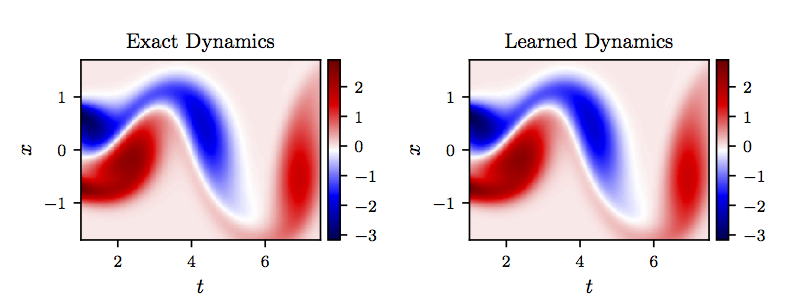
Navier-Stokes equation: A randomly picked snapshot of a solution to the Navier-Stokes equation (left panel) is compared to the corresponding snapshot of the solution of the learned partial differential equation (right panel). The identified system correctly captures the form of the dynamics and accurately reproduces the solution with a relative L2-error of 5.79e-03 in space and time.

Conclusion

We have presented a deep learning approach for extracting nonlinear partial differential equations from spatio-temporal datasets. The proposed algorithm leverages recent developments in automatic differentiation to construct efficient algorithms for learning infinite dimensional dynamical systems using deep neural networks. In order to validate the performance of our approach we had no other choice than to rely on black-box solvers. This signifies the importance of developing general purpose partial differential equation solvers. Developing these types of solvers is still in its infancy and more collaborative work is needed to bring them to the maturity level of conventional methods such as finite elements, finite differences, and spectral methods which have been around for more than half a century or so.

There exist a series of open questions mandating further investigations. For instance, many real-world partial differential equations depend on parameters and, when the parameters are varied, they may go through bifurcations (e.g., the Reynold number for the Navier-Stokes equations). Here, the goal would be to collect data from the underlying dynamics corresponding to various parameter values, and infer the parameterized partial differential equation. Another exciting avenue of future research would be to apply convolutional architectures for mitigating the complexity associated with partial differential equations with very high-dimensional inputs. These types of equations appear routinely in dynamic programming, optimal control, or reinforcement learning. Moreover, a quick look at the list of nonlinear partial differential equations on Wikipedia reveals that many of these equations take the form considered in this work. However, a handful of them do not take this form, including the Boussinesq type equation $u_{tt} - u_{xx} - 2 \alpha (u u_x)_x - \beta u_{xxtt} = 0$ . It would be interesting to extend the framework outlined in the current work to incorporate all such cases. In the end, it is not always clear what measurements of a dynamical system to take. Even if we did know, collecting these measurements might be prohibitively expensive. It is well-known that time-delay coordinates of a single variable can act as additional variables. It might be interesting to investigating this idea for the infinite dimensional setting of partial differential equations.

Acknowledgements

This work received support by the DARPA EQUiPS grant N66001-15-2-4055 and the AFOSR grant FA9550-17-1-0013. All data and codes are publicly available on GitHub.

Citation

@article{raissi2018deep,
  title={Deep Hidden Physics Models: Deep Learning of Nonlinear Partial Differential Equations},
  author={Raissi, Maziar},
  journal={arXiv preprint arXiv:1801.06637},
  year={2018}
}