Authors

Maziar Raissi, Paris Perdikaris, and George Em Karniadakis

Abstract

We introduce physics informed neural networks – neural networks that are trained to solve supervised learning tasks while respecting any given law of physics described by general nonlinear partial differential equations. We present our developments in the context of solving two main classes of problems: data-driven solution and data-driven discovery of partial differential equations. Depending on the nature and arrangement of the available data, we devise two distinct classes of algorithms, namely continuous time and discrete time models. The resulting neural networks form a new class of data-efficient universal function approximators that naturally encode any underlying physical laws as prior information. In the first part, we demonstrate how these networks can be used to infer solutions to partial differential equations, and obtain physics-informed surrogate models that are fully differentiable with respect to all input coordinates and free parameters. In the second part, we focus on the problem of data-driven discovery of partial differential equations.

Data-driven Solutions of Nonlinear Partial Differential Equations

In this first part of our two-part treatise, we focus on computing data-driven solutions to partial differential equations of the general form

$u_t + \mathcal{N}[u] = 0,\ x \in \Omega, \ t\in[0,T],$

where $u(t,x)$ denotes the latent (hidden) solution, $\mathcal{N}[\cdot]$ is a nonlinear differential operator, and $\Omega$ is a subset of $\mathbb{R}^D$ . In what follows, we put forth two distinct classes of algorithms, namely continuous and discrete time models, and highlight their properties and performance through the lens of different benchmark problems. All code and data-sets are available here.

Continuous Time Models

We define $f(t,x)$ to be given by

$f := u_t + \mathcal{N}[u],$

Example (Burgers’ Equation)

As an example, let us consider the Burgers’ equation. In one space dimension, the Burger’s equation along with Dirichlet boundary conditions reads as

$\begin{array}{l} u_t + u u_x - (0.01/\pi) u_{xx} = 0,\ \ \ x \in [-1,1],\ \ \ t \in [0,1],\\ u(0,x) = -\sin(\pi x),\\ u(t,-1) = u(t,1) = 0. \end{array}$

Let us define $f(t,x)$ to be given by

$f := u_t + u u_x - (0.01/\pi) u_{xx},$

and proceed by approximating $u(t,x)$ by a deep neural network. To highlight the simplicity in implementing this idea let us include a Python code snippet using Tensorflow. To this end, $u(t,x)$ can be simply defined as

def u(t, x):
    u = neural_net(tf.concat([t,x],1), weights, biases)
    return u

Correspondingly, the physics informed neural network $f(t,x)$ takes the form

def f(t, x):
    u = u(t, x)
    u_t = tf.gradients(u, t)[0]
    u_x = tf.gradients(u, x)[0]
    u_xx = tf.gradients(u_x, x)[0]
    f = u_t + u*u_x - (0.01/tf.pi)*u_xx
    return f

The shared parameters between the neural networks $u(t,x)$ and $f(t,x)$ can be learned by minimizing the mean squared error loss

$MSE = MSE_u + MSE_f,$

where

$MSE_u = \frac{1}{N_u}\sum_{i=1}^{N_u} |u(t^i_u,x_u^i) - u^i|^2,$

and

$MSE_f = \frac{1}{N_f}\sum_{i=1}^{N_f}|f(t_f^i,x_f^i)|^2.$

Here, $\{t_u^i, x_u^i, u^i\}_{i=1}^{N_u}$ denote the initial and boundary training data on $u(t,x)$ and $\{t_f^i, x_f^i\}_{i=1}^{N_f}$ specify the collocations points for $f(t,x)$ . The loss $MSE_u$ corresponds to the initial and boundary data while $MSE_f$ enforces the structure imposed by the Burgers’ equation at a finite set of collocation points.

The following figure summarizes our results for the data-driven solution of the Burgers’ equation.

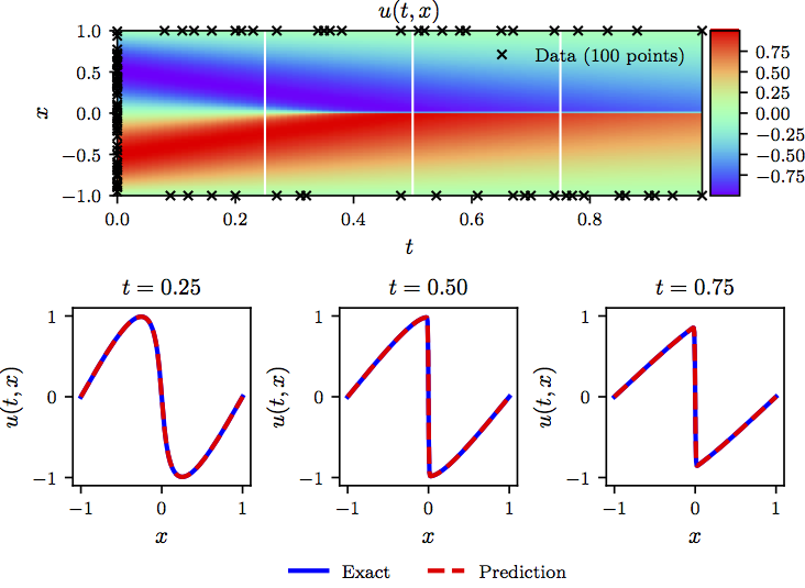
Burgers’ equation: Top: Predicted solution along with the initial and boundary training data. In addition we are using 10,000 collocation points generated using a Latin Hypercube Sampling strategy. Bottom: Comparison of the predicted and exact solutions corresponding to the three temporal snapshots depicted by the white vertical lines in the top panel. Model training took approximately 60 seconds on a single NVIDIA Titan X GPU card.

Example (Shrödinger Equation)

This example aims to highlight the ability of our method to handle periodic boundary conditions, complex-valued solutions, as well as different types of nonlinearities in the governing partial differential equations. The nonlinear Schrödinger equation along with periodic boundary conditions is given by

$\begin{array}{l} i h_t + 0.5 h_{xx} + |h|^2 h = 0,\ \ \ x \in [-5, 5],\ \ \ t \in [0, \pi/2],\\ h(0,x) = 2\ \text{sech}(x),\\ h(t,-5) = h(t, 5),\\ h_x(t,-5) = h_x(t, 5), \end{array}$

where $h(t,x)$ is the complex-valued solution. Let us define $f(t,x)$ to be given by

$f := i h_t + 0.5 h_{xx} + |h|^2 h,$

and proceed by placing a complex-valued neural network prior on $h(t,x)$ . In fact, if $u$ denotes the real part of $h$ and $v$ is the imaginary part, we are placing a multi-out neural network prior on $h(t,x) = \begin{bmatrix} u(t,x) & v(t,x) \end{bmatrix}$ . This will result in the complex-valued (multi-output) physic informed neural network $f(t,x)$ . The shared parameters of the neural networks $h(t,x)$ and $f(t,x)$ can be learned by minimizing the mean squared error loss

$MSE = MSE_0 + MSE_b + MSE_f,$

where

$MSE_0 = \frac{1}{N_0}\sum_{i=1}^{N_0} |h(0,x_0^i) - h^i_0|^2,$ $MSE_b = \frac{1}{N_b}\sum_{i=1}^{N_b} \left(|h^i(t^i_b,-5) - h^i(t^i_b,5)|^2 + |h^i_x(t^i_b,-5) - h^i_x(t^i_b,5)|^2\right),$

and

$MSE_f = \frac{1}{N_f}\sum_{i=1}^{N_f}|f(t_f^i,x_f^i)|^2.$

Here, $\{x_0^i, h^i_0\}_{i=1}^{N_0}$ denotes the initial data, $\{t^i_b\}_{i=1}^{N_b}$ corresponds to the collocation points on the boundary, and $\{t_f^i,x_f^i\}_{i=1}^{N_f}$ represents the collocation points on $f(t,x)$ . Consequently, $MSE_0$ corresponds to the loss on the initial data, $MSE_b$ enforces the periodic boundary conditions, and $MSE_f$ penalizes the Schrödinger equation not being satisfied on the collocation points.

The following figure summarizes the results of our experiment.

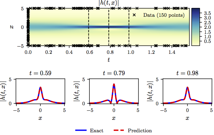
Shrödinger equation: Top: Predicted solution along with the initial and boundary training data. In addition we are using 20,000 collocation points generated using a Latin Hypercube Sampling strategy. Bottom: Comparison of the predicted and exact solutions corresponding to the three temporal snapshots depicted by the dashed vertical lines in the top panel.

One potential limitation of the continuous time neural network models considered so far, stems from the need to use a large number of collocation points $N_f$ in order to enforce physics informed constraints in the entire spatio-temporal domain. Although this poses no significant issues for problems in one or two spatial dimensions, it may introduce a severe bottleneck in higher dimensional problems, as the total number of collocation points needed to globally enforce a physics informed constrain (i.e., in our case a partial differential equation) will increase exponentially. In the next section, we put forth a different approach that circumvents the need for collocation points by introducing a more structured neural network representation leveraging the classical Runge-Kutta time-stepping schemes.

Discrete Time Models

Let us employ the general form of Runge-Kutta methods with $q$ stages and obtain

$\begin{array}{ll} u^{n+c_i} = u^n - \Delta t \sum_{j=1}^q a_{ij} \mathcal{N}[u^{n+c_j}], \ \ i=1,\ldots,q,\\ u^{n+1} = u^{n} - \Delta t \sum_{j=1}^q b_j \mathcal{N}[u^{n+c_j}]. \end{array}$

Here, $u^{n+c_j}(x) = u(t^n + c_j \Delta t, x)$ for $j=1, \ldots, q$ . This general form encapsulates both implicit and explicit time-stepping schemes, depending on the choice of the parameters $\{a_{ij},b_j,c_j\}$ . The above equations can be equivalently expressed as

$\begin{array}{ll} u^{n} = u^n_i, \ \ i=1,\ldots,q,\\ u^n = u^n_{q+1}, \end{array}$

where

$\begin{array}{ll} u^n_i := u^{n+c_i} + \Delta t \sum_{j=1}^q a_{ij} \mathcal{N}[u^{n+c_j}], \ \ i=1,\ldots,q,\\ u^n_{q+1} := u^{n+1} + \Delta t \sum_{j=1}^q b_j \mathcal{N}[u^{n+c_j}]. \end{array}$

We proceed by placing a multi-output neural network prior on

$\begin{bmatrix} u^{n+c_1}(x), \ldots, u^{n+c_q}(x), u^{n+1}(x) \end{bmatrix}.$

This prior assumption along with the above equations result in a physics informed neural network that takes $x$ as an input and outputs

$\begin{bmatrix} u^n_1(x), \ldots, u^n_q(x), u^n_{q+1}(x) \end{bmatrix}.$

Example (Allen-Cahn Equation)

This example aims to highlight the ability of the proposed discrete time models to handle different types of nonlinearity in the governing partial differential equation. To this end, let us consider the Allen-Cahn equation along with periodic boundary conditions

$\begin{array}{l} u_t - 0.0001 u_{xx} + 5 u^3 - 5 u = 0, \ \ \ x \in [-1,1], \ \ \ t \in [0,1],\\ u(0, x) = x^2 \cos(\pi x),\\ u(t,-1) = u(t,1),\\ u_x(t,-1) = u_x(t,1). \end{array}$

The Allen-Cahn equation is a well-known equation from the area of reaction-diffusion systems. It describes the process of phase separation in multi-component alloy systems, including order-disorder transitions. For the Allen-Cahn equation, the nonlinear operator is given by

$\mathcal{N}[u^{n+c_j}] = -0.0001 u^{n+c_j}_{xx} + 5 \left(u^{n+c_j}\right)^3 - 5 u^{n+c_j},$

and the shared parameters of the neural networks can be learned by minimizing the sum of squared errors

$SSE = SSE_n + SSE_b,$

where

$SSE_n = \sum_{j=1}^{q+1} \sum_{i=1}^{N_n} |u^n_j(x^{n,i}) - u^{n,i}|^2,$

and

$\begin{array}{rl} SSE_b =& \sum_{i=1}^q |u^{n+c_i}(-1) - u^{n+c_i}(1)|^2 + |u^{n+1}(-1) - u^{n+1}(1)|^2 \\ +& \sum_{i=1}^q |u_x^{n+c_i}(-1) - u_x^{n+c_i}(1)|^2 + |u_x^{n+1}(-1) - u_x^{n+1}(1)|^2. \end{array}$

Here, $\{x^{n,i}, u^{n,i}\}_{i=1}^{N_n}$ corresponds to the data at time $t^n$ .

The following figure summarizes our predictions after the network has been trained using the above loss function.

Allen-Cahn equation: Top: Solution along with the location of the initial training snapshot at t=0.1 and the final prediction snapshot at t=0.9. Bottom: Initial training data and final prediction at the snapshots depicted by the white vertical lines in the top panel.

Data-driven Discovery of Nonlinear Partial Differential Equations

In this second part of our study, we shift our attention to the problem of data-driven discovery of partial differential equations. To this end, let us consider parametrized and nonlinear partial differential equations of the general form

$u_t + \mathcal{N}[u;\lambda] = 0,\ x \in \Omega, \ t\in[0,T],$

where $u(t,x)$ denotes the latent (hidden) solution, $\mathcal{N}[\cdot;\lambda]$ is a nonlinear operator parametrized by $\lambda$ , and $\Omega$ is a subset of $\mathbb{R}^D$ . Now, the problem of data-driven discovery of partial differential equations poses the following question: given a small set of scattered and potentially noisy observations of the hidden state $u(t,x)$ of a system, what are the parameters $\lambda$ that best describe the observed data?

In what follows, we will provide an overview of our two main approaches to tackle this problem, namely continuous time and discrete time models, as well as a series of results and systematic studies for a diverse collection of benchmarks. In the first approach, we will assume availability of scattered and potential noisy measurements across the entire spatio-temporal domain. In the latter, we will try to infer the unknown parameters $\lambda$ from only two data snapshots taken at distinct time instants. All data and codes used in this manuscript are publicly available on GitHub.

Continuous Time Models

We define $f(t,x)$ to be given by

$f := u_t + \mathcal{N}[u;\lambda],\label{eq:PDE_RHS}$

and proceed by approximating $u(t,x)$ by a deep neural network. This assumption results in a physics informed neural network $f(t,x)$ . This network can be derived by the calculus on computational graphs: Backpropagation. It is worth highlighting that the parameters of the differential operator $\lambda$ turn into parameters of the physics informed neural network $f(t,x)$ .

Example (Navier-Stokes Equation)

Our next example involves a realistic scenario of incompressible fluid flow as described by the ubiquitous Navier-Stokes equations. Navier-Stokes equations describe the physics of many phenomena of scientific and engineering interest. They may be used to model the weather, ocean currents, water flow in a pipe and air flow around a wing. The Navier-Stokes equations in their full and simplified forms help with the design of aircraft and cars, the study of blood flow, the design of power stations, the analysis of the dispersion of pollutants, and many other applications. Let us consider the Navier-Stokes equations in two dimensions (2D) given explicitly by

$\begin{array}{c} u_t + \lambda_1 (u u_x + v u_y) = -p_x + \lambda_2(u_{xx} + u_{yy}),\\ v_t + \lambda_1 (u v_x + v v_y) = -p_y + \lambda_2(v_{xx} + v_{yy}), \end{array}$

where $u(t, x, y)$ denotes the $x$ -component of the velocity field, $v(t, x, y)$ the $y$ -component, and $p(t, x, y)$ the pressure. Here, $\lambda = (\lambda_1, \lambda_2)$ are the unknown parameters. Solutions to the Navier-Stokes equations are searched in the set of divergence-free functions; i.e.,

$u_x + v_y = 0.$

This extra equation is the continuity equation for incompressible fluids that describes the conservation of mass of the fluid. We make the assumption that

$u = \psi_y,\ \ \ v = -\psi_x,$

for some latent function $\psi(t,x,y)$ . Under this assumption, the continuity equation will be automatically satisfied. Given noisy measurements

$\{t^i, x^i, y^i, u^i, v^i\}_{i=1}^{N}$

of the velocity field, we are interested in learning the parameters $\lambda$ as well as the pressure $p(t,x,y)$ . We define $f(t,x,y)$ and $g(t,x,y)$ to be given by

$\begin{array}{c} f := u_t + \lambda_1 (u u_x + v u_y) + p_x - \lambda_2(u_{xx} + u_{yy}),\\ g := v_t + \lambda_1 (u v_x + v v_y) + p_y - \lambda_2(v_{xx} + v_{yy}), \end{array}$

and proceed by jointly approximating $\begin{bmatrix} \psi(t,x,y) & p(t,x,y) \end{bmatrix}$ using a single neural network with two outputs. This prior assumption results into a physics informed neural network $\begin{bmatrix} f(t,x,y) & g(t,x,y) \end{bmatrix}$ . The parameters $\lambda$ of the Navier-Stokes operator as well as the parameters of the neural networks $\begin{bmatrix} \psi(t,x,y) & p(t,x,y) \end{bmatrix}$ and $\begin{bmatrix} f(t,x,y) & g(t,x,y) \end{bmatrix}$ can be trained by minimizing the mean squared error loss

$\begin{array}{rl} MSE :=& \frac{1}{N}\sum_{i=1}^{N} \left(|u(t^i,x^i,y^i) - u^i|^2 + |v(t^i,x^i,y^i) - v^i|^2\right) \\ +& \frac{1}{N}\sum_{i=1}^{N} \left(|f(t^i,x^i,y^i)|^2 + |g(t^i,x^i,y^i)|^2\right). \end{array}$

A summary of our results for this example is presented in the following figures.

Navier-Stokes equation: Top: Incompressible flow and dynamic vortex shedding past a circular cylinder at Re=100. The spatio-temporal training data correspond to the depicted rectangular region in the cylinder wake. Bottom: Locations of training data-points for the the stream-wise and transverse velocity components.

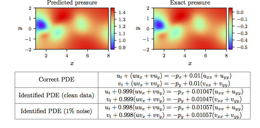
Navier-Stokes equation: Top: Predicted versus exact instantaneous pressure field at a representative time instant. By definition, the pressure can be recovered up to a constant, hence justifying the different magnitude between the two plots. This remarkable qualitative agreement highlights the ability of physics-informed neural networks to identify the entire pressure field, despite the fact that no data on the pressure are used during model training. Bottom: Correct partial differential equation along with the identified one.

Our approach so far assumes availability of scattered data throughout the entire spatio-temporal domain. However, in many cases of practical interest, one may only be able to observe the system at distinct time instants. In the next section, we introduce a different approach that tackles the data-driven discovery problem using only two data snapshots. We will see how, by leveraging the classical Runge-Kutta time-stepping schemes, one can construct discrete time physics informed neural networks that can retain high predictive accuracy even when the temporal gap between the data snapshots is very large.

Discrete Time Models

We begin by employing the general form of Runge-Kutta methods with $q$ stages and obtain

$\begin{array}{ll} u^{n+c_i} = u^n - \Delta t \sum_{j=1}^q a_{ij} \mathcal{N}[u^{n+c_j};\lambda], \ \ i=1,\ldots,q,\\ u^{n+1} = u^{n} - \Delta t \sum_{j=1}^q b_j \mathcal{N}[u^{n+c_j};\lambda]. \end{array}$

$\begin{array}{ll} u^{n} = u^n_i, \ \ i=1,\ldots,q,\\ u^{n+1} = u^{n+1}_{i}, \ \ i=1,\ldots,q. \end{array}$

where

$\begin{array}{ll} u^n_i := u^{n+c_i} + \Delta t \sum_{j=1}^q a_{ij} \mathcal{N}[u^{n+c_j};\lambda], \ \ i=1,\ldots,q,\\ u^{n+1}_{i} := u^{n+c_i} + \Delta t \sum_{j=1}^q (a_{ij} - b_j) \mathcal{N}[u^{n+c_j};\lambda], \ \ i=1,\ldots,q. \end{array}$

We proceed by placing a multi-output neural network prior on

$\begin{bmatrix} u^{n+c_1}(x), \ldots, u^{n+c_q}(x) \end{bmatrix}.$

This prior assumption result in two physics informed neural networks

$\begin{bmatrix} u^{n}_1(x), \ldots, u^{n}_q(x), u^{n}_{q+1}(x) \end{bmatrix},$

and

$\begin{bmatrix} u^{n+1}_1(x), \ldots, u^{n+1}_q(x), u^{n+1}_{q+1}(x) \end{bmatrix}.$

Given noisy measurements at two distinct temporal snapshots $\{\mathbf{x}^{n}, \mathbf{u}^{n}\}$ and $\{\mathbf{x}^{n+1}, \mathbf{u}^{n+1}\}$ of the system at times $t^{n}$ and $t^{n+1}$ , respectively, the shared parameters of the neural networks along with the parameters $\lambda$ of the differential operator can be trained by minimizing the sum of squared errors

$SSE = SSE_n + SSE_{n+1},$

where

$SSE_n := \sum_{j=1}^q \sum_{i=1}^{N_n} |u^n_j(x^{n,i}) - u^{n,i}|^2,$

and

$SSE_{n+1} := \sum_{j=1}^q \sum_{i=1}^{N_{n+1}} |u^{n+1}_j(x^{n+1,i}) - u^{n+1,i}|^2.$

Here, $\mathbf{x}^n = \left\{x^{n,i}\right\}_{i=1}^{N_n}$ , $\mathbf{u}^n = \left\{u^{n,i}\right\}_{i=1}^{N_n}$ , $\mathbf{x}^{n+1} = \left\{x^{n+1,i}\right\}_{i=1}^{N_{n+1}}$ , and $\mathbf{u}^{n+1} = \left\{u^{n+1,i}\right\}_{i=1}^{N_{n+1}}$ .

Example (Korteweg–de Vries Equation)

Our final example aims to highlight the ability of the proposed framework to handle governing partial differential equations involving higher order derivatives. Here, we consider a mathematical model of waves on shallow water surfaces; the Korteweg-de Vries (KdV) equation. The KdV equation reads as

$u_t + \lambda_1 u u_x + \lambda_2 u_{xxx} = 0,$

with $(\lambda_1, \lambda_2)$ being the unknown parameters. For the KdV equation, the nonlinear operator is given by

$\mathcal{N}[u^{n+c_j}] = \lambda_1 u^{n+c_j} u^{n+c_j}_x - \lambda_2 u^{n+c_j}_{xxx}$

and the shared parameters of the neural networks along with the parameters $\lambda = (\lambda_1, \lambda_2)$ of the KdV equation can be learned by minimizing the sum of squared errors given above.

The results of this experiment are summarized in the following figure.

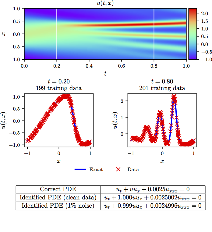
KdV equation: Top: Solution along with the temporal locations of the two training snapshots. Middle: Training data and exact solution corresponding to the two temporal snapshots depicted by the dashed vertical lines in the top panel. Bottom: Correct partial differential equation along with the identified one.

Conclusion

Although a series of promising results was presented, the reader may perhaps agree that this two-part treatise creates more questions than it answers. In a broader context, and along the way of seeking further understanding of such tools, we believe that this work advocates a fruitful synergy between machine learning and classical computational physics that has the potential to enrich both fields and lead to high-impact developments.

Acknowledgements

This work received support by the DARPA EQUiPS grant N66001-15-2-4055 and the AFOSR grant FA9550-17-1-0013. All data and codes are publicly available on GitHub.

Citation

@article{raissi2019physics,
  title={Physics-informed neural networks: A deep learning framework for solving forward and inverse problems involving nonlinear partial differential equations},
  author={Raissi, Maziar and Perdikaris, Paris and Karniadakis, George E},
  journal={Journal of Computational Physics},
  volume={378},
  pages={686--707},
  year={2019},
  publisher={Elsevier}
}

@article{raissi2017physicsI,
  title={Physics Informed Deep Learning (Part I): Data-driven Solutions of Nonlinear Partial Differential Equations},
  author={Raissi, Maziar and Perdikaris, Paris and Karniadakis, George Em},
  journal={arXiv preprint arXiv:1711.10561},
  year={2017}
}

@article{raissi2017physicsII,
  title={Physics Informed Deep Learning (Part II): Data-driven Discovery of Nonlinear Partial Differential Equations},
  author={Raissi, Maziar and Perdikaris, Paris and Karniadakis, George Em},
  journal={arXiv preprint arXiv:1711.10566},
  year={2017}
}

Physics Informed Deep Learning

Data-driven solutions and discovery of Nonlinear Partial Differential Equations

Authors

Abstract

Data-driven Solutions of Nonlinear Partial Differential Equations

Continuous Time Models

Discrete Time Models

Data-driven Discovery of Nonlinear Partial Differential Equations

Continuous Time Models

Discrete Time Models

Citation