Forward Backward Stochastic Neural Networks

Classical numerical methods for solving partial differential equations suffer from the curse of dimensionality mainly due to their reliance on meticulously generated spatio-temporal grids. Inspired by modern deep learning based techniques for solving forward and inverse problems associated with partial differential equations, we circumvent the tyranny of numerical discretization by devising an algorithm that is scalable to high-dimensions. In particular, we approximate the unknown solution by a deep neural network which essentially enables us to benefit from the merits of automatic differentiation. To train the aforementioned neural network we leverage the well-known connection between high-dimensional partial differential equations and forward-backward stochastic differential equations. In fact, independent realizations of a standard Brownian motion will act as training data. We test the effectiveness of our approach for a couple of benchmark problems spanning a number of scientific domains including Black-Scholes-Barenblatt and Hamilton-Jacobi-Bellman equations, both in 100-dimensions.

Problem Setup and Solution Methodology

In this work, we consider coupled forward-backward stochastic differential equations of the general form

where \(W_t\) is a vector-valued Brownian motion. A solution to these equations consists of the stochastic processes \(X_t\), \(Y_t\), and \(Z_t\). It is well-known that coupled forward-backward stochastic differential equations are related to quasi-linear partial differential equations of the form

with terminal condition \(u(T,x) = g(x)\), where \(u(t,x)\) is the unknown solution and

Here, \(Du\) and \(D^2u\) denote the gradient vector and the Hessian matrix of \(u\), respectively. In particular, it follows directly from Ito’s formula that solutions of forward-backward stochastic differential equations and quasi-linear partial differential equations are related according to

Inspired by recent developments in physics-informed deep learning and deep hidden physics models, we proceed by approximating the unknown solution \(u(t,x)\) by a deep neural network. We obtain the required gradient vector \(Du(t,x)\) by applying the chain rule for differentiating compositions of functions using automatic differentiation. In particular, to compute the derivatives we rely on Tensorflow which is a popular and relatively well documented open source software library for automatic differentiation and deep learning computations.

Parameters of the neural network representing \(u(t,x)\) can be learned by minimizing the following loss function obtained from discretizing the forward-backward stochastic differential equation using the standard Euler-Maruyama scheme. To be more specific, let us employ the Euler-Maruyama scheme and obtain

for \(n = 0, 1, \ldots, N-1\), where \(\Delta t^n := t^{n+1} - t^n = T/N\) and \(\Delta W^n \sim \mathcal{N}(0, \Delta t^n)\) is a random variable with mean \(0\) and standard deviation \(\sqrt{\Delta t^n}\). The loss function is then given by

which corresponds to \(M\) different realizations of the underlying Brownian motion. Here, \(\Phi^n_m := \varphi(t^n,X^n_m,Y^n_m,Z^n_m)\) and \(\Sigma^n_m := \sigma(t^n,X^n_m,Y^n_m)\). The subscript \(m\) corresponds to the \(m\)-th realization of the underlying Brownian motion while the superscript \(n\) corresponds to time \(t^n\). It is worth recalling that \(Y_m^n = u(t^n, X_m^n)\) and \(Z_m^n = D u(t^n, X_m^n)\), and consequently the loss is a function of the parameters of the neural network \(u(t,x)\). Furthermore, we have

and \(X^0_m = \xi\) for every \(m\).

Results

The proposed framework provides a universal treatment of coupled forward-backward stochastic differential equations of fundamentally different nature and their corresponding high-dimensional partial differential equations. This generality will be demonstrated by applying the algorithm to a wide range of canonical problems spanning a number of scientific domains including a 100-dimensional Black-Scholes-Barenblatt equation and a 100-dimensional Hamilton-Jacobi-Bellman equation. These examples are motivated by the pioneering work of Beck et. al.. All data and codes used in this manuscript will be publicly available on GitHub.

Black-Scholes-Barenblatt Equation in 100D

Let us start with the following forward-backward stochastic differential equations

where \(T=1\), \(\sigma = 0.4\), \(r=0.05\), \(\xi = (1,0.5,1,0.5,\ldots,1,0.5) \in \mathbb{R}^{100}\), and \(g(x) = \Vert x \Vert ^2\). The above equations are related to the Black-Scholes-Barenblatt equation

with terminal condition \(u(T,x) = g(x)\). This equation admits the explicit solution

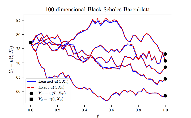
which can be used to test the accuracy of the proposed algorithm. We approximate the unknown solution \(u(t,x)\) by a 5-layer deep neural network with \(256\) neurons per hidden layer. Furthermore, we partition the time domain \([0,T]\) into \(N=50\) equally spaced intervals. Upon minimizing the loss function, using the Adam optimizer with mini-batches of size \(100\) (i.e., \(100\) realizations of the underlying Brownian motion), we obtain the results reported in the following figure. In this figure, we are evaluating the learned solution \(Y_t = u(t,X_t)\) at representative realizations (not seen during training) of the underlying high-dimensional process \(X_t\). Unlike the state of the art algorithms, which can only approximate \(Y_0 = u(0,X_0)\) at time \(0\) and at the initial spatial point \(X_0=\xi\), our algorithm is capable of approximating the entire solution function \(u(t,x)\) in a single round of training as demonstrated in the following figure.

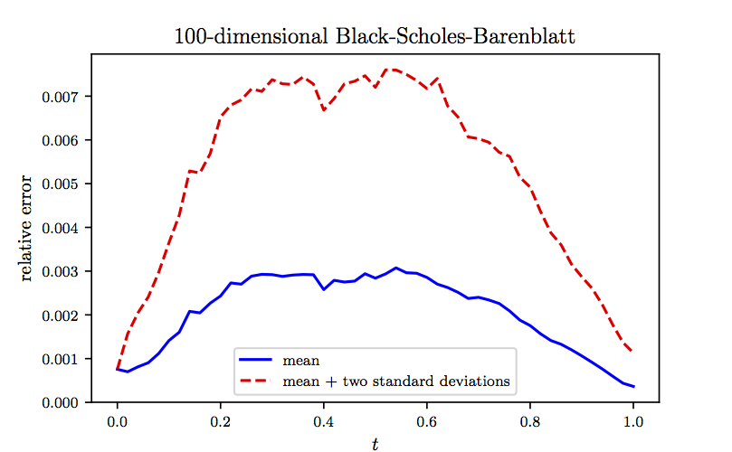
To further scrutinize the performance of our algorithm, in the following figure we report the mean and mean plus two standard deviations of the relative errors between model predictions and the exact solution computed based on \(100\) independent realizations of the underlying Brownian motion. It is worth noting that in the previous figure we were plotting \(5\) representative examples of the \(100\) realizations used to generate the following figure. The results reported in these two figures are obtained after \(2 \times 10^4\), \(3 \times 10^4\), \(3 \times 10^4\), and \(2 \times 10^4\) consecutive iterations of the Adam optimizer with learning rates of \(10^{-3}\), \(10^{-4}\), \(10^{-5}\), and \(10^{-6}\), respectively. The total number of iterations is therefore given by \(10^5\). Every \(10\) iterations of the optimizer takes about \(0.88\) seconds on a single NVIDIA Titan X GPU card. In each iteration of the Adam optimizer we are using \(100\) different realizations of the underlying Brownian motion. Consequently, the total number of Brownian motion trajectories observed by the algorithm is given by \(10^7\). It is worth highlighting that the algorithm converges to the exact value \(Y_0 = u(0,X_0)\) in the first few hundred iterations of the Adam optimizer. For instance after only \(500\) steps of training, the algorithms achieves an accuracy of around \(2.3 \times 10^{-3}\) in terms of relative error. This is comparable to the results reported here, both in terms of accuracy and the speed of the algorithm. However, to obtain more accurate estimates for \(Y_t = u(t,X_t)\) at later times \(t>0\) we need to train the algorithm using more iterations of the Adam optimizer.

Hamilton-Jacobi-Bellman Equation in 100D

Let us now consider the following forward-backward stochastic differential equations

where \(T=1\), \(\sigma = \sqrt{2}\), \(\xi = (0,0,\ldots,0)\in \mathbb{R}^{100}\), and \(g(x) = \ln\left(0.5\left(1+\Vert x\Vert^2\right)\right)\). The above equations are related to the Hamilton-Jacobi-Bellman equation

with terminal condition \(u(T,x) = g(x)\). This equation admits the explicit solution

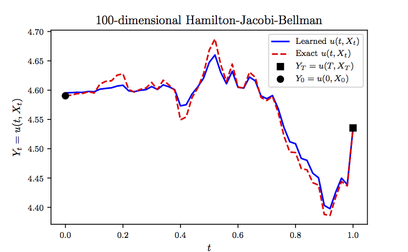
which can be used to test the accuracy of the proposed algorithm. In fact, due to the presence of the expectation operator \(\mathbb{E}\) in the above equation, we can only approximately compute the exact solution. To be precise, we use \(10^5\) Monte-Carlo samples to approximate the exact solution and use the result as ground truth. We represent the unknown solution \(u(t,x)\) by a \(5\)-layer deep neural network with \(256\) neurons per hidden layer. Furthermore, we partition the time domain \([0,T]\) into \(N=50\) equally spaced intervals. Upon minimizing the loss function, using the Adam optimizer with mini-batches of size \(100\) (i.e., \(100\) realizations of the underlying Brownian motion), we obtain the results reported in the following figure. In this figure, we are evaluating the learned solution \(Y_t = u(t,X_t)\) at a representative realization (not seen during training) of the underlying high-dimensional process \(X_t\). It is worth noting that computing the exact solution to this problem is prohibitively costly due to the need for the aforementioned Monte-Carlo sampling strategy. That is why we are depicting only a single realization of the solution trajectories in the following figure. Unlike the state of the art algorithms, which can only approximate \(Y_0 = u(0,X_0)\) at time \(0\) and at the initial spatial point \(X_0=\xi\), our algorithm is capable of approximating the entire solution function \(u(t,x)\) in a single round of training as demonstrated in the following figure.

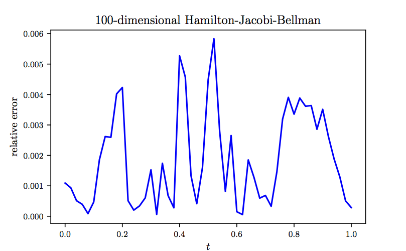
To further investigate the performance of our algorithm, in the following figure we report the relative error between model prediction and the exact solution computed for the same realization of the underlying Brownian motion as the one used in the previous figure. The results reported in these two figures are obtained after \(2 \times 10^4\), \(3 \times 10^4\), \(3 \times 10^4\), and \(2 \times 10^4\) consecutive iterations of the Adam optimizer with learning rates of \(10^{-3}\), \(10^{-4}\), \(10^{-5}\), and \(10^{-6}\), respectively. The total number of iterations is therefore given by \(10^5\). Every \(10\) iterations of the optimizer takes about \(0.79\) seconds on a single NVIDIA Titan X GPU card. In each iteration of the Adam optimizer we are using \(100\) different realizations of the underlying Brownian motion. Consequently, the total number of Brownian motion trajectories observed by the algorithm is given by \(10^7\). It is worth highlighting that the algorithm converges to the exact value \(Y_0 = u(0,X_0)\) in the first few hundred iterations of the Adam optimizer. For instance after only \(100\) steps of training, the algorithms achieves an accuracy of around \(7.3 \times 10^{-3}\) in terms of relative error. This is comparable to the results reported here, both in terms of accuracy and the speed of the algorithm. However, to obtain more accurate estimates for \(Y_t = u(t,X_t)\) at later times \(t>0\) we need to train the algorithm using more iterations of the Adam optimizer.

Summary and Discussion

In this work, we put forth a deep learning approach for solving coupled forward-backward stochastic differential equations and their corresponding high-dimensional partial differential equations. The resulting methodology showcases a series of promising results for a diverse collection of benchmark problems. As deep learning technology is continuing to grow rapidly both in terms of methodological, algorithmic, and infrastructural developments, we believe that this is a timely contribution that can benefit practitioners across a wide range of scientific domains. Specific applications that can readily enjoy these benefits include, but are not limited to, stochastic control, theoretical economics, and mathematical finance.

In terms of future work, one could straightforwardly extend the proposed framework in the current work to solve second-order backward stochastic differential equations. The key is to leverage the fundamental relationships between second-order backward stochastic differential equations and fully-nonlinear second-order partial differential equations. Moreover, our method can be used to solve stochastic control problems, where in general, to obtain a candidate for an optimal control, one needs to solve a coupled forward-backward stochastic differential equation, where the backward components influence the dynamics of the forward component.

Acknowledgements

This work received support by the DARPA EQUiPS grant N66001-15-2-4055 and the AFOSR grant FA9550-17-1-0013. All data and codes are publicly available on GitHub.

Citation

@article{raissi2018forwardbackward,
  title={Forward-Backward Stochastic Neural Networks: Deep Learning of High-dimensional Partial Differential Equations},
  author={Raissi, Maziar},
  journal={arXiv preprint arXiv:1804.07010},
  year={2018}
}