Multistep Neural Networks
Data-driven Discovery of Nonlinear Dynamical Systems
The process of transforming observed data into predictive mathematical models of the physical world has always been paramount in science and engineering. Although data is currently being collected at an ever-increasing pace, devising meaningful models out of such observations in an automated fashion still remains an open problem. In this work, we put forth a machine learning approach for identifying nonlinear dynamical systems from data. Specifically, we blend classical tools from numerical analysis, namely the multi-step time-stepping schemes, with powerful nonlinear function approximators, namely deep neural networks, to distill the mechanisms that govern the evolution of a given data-set. We test the effectiveness of our approach for several benchmark problems involving the identification of complex, nonlinear and chaotic dynamics, and we demonstrate how this allows us to accurately learn the dynamics, forecast future states, and identify basins of attraction. In particular, we study the Lorenz system, the fluid flow behind a cylinder, the Hopf bifurcation, and the Glycoltic oscillator model as an example of complicated nonlinear dynamics typical of biological systems.
Problem setup and solution methodology
In this work, we consider nonlinear dynamical systems of the form
\[\frac{d}{d t} \mathbf{x}(t) = \mathbf{f}\left(\mathbf{x}(t)\right),\]where the vector \(\mathbf{x}(t) \in \mathbb{R}^D\) denotes the state of the system at time \(t\) and the function \(\mathbf{f}\) describes the evolution of the system. Given noisy measurements of the state \(\mathbf{x}(t)\) of the system at several time instances \(t_1, t_2, \ldots, t_N\), our goal is to determine the function \(\mathbf{f}\) and consequently discover the underlying dynamical system from data. We proceed by employing the general form of a linear multistep method with \(M\) steps to obtain
\[\sum_{m=0}^M \left[\alpha_m \mathbf{x}_{n-m} + \Delta t \beta_m \mathbf{f}(\mathbf{x}_{n-m})\right] = 0, \ \ \ n = M, \ldots, N.\]Here, \(\mathbf{x}_{n-m}\) denotes the state of the system \(\mathbf{x}(t_{n-m})\) at time \(t_{n-m}\). Different choices for the parameters \(\alpha_m\) and \(\beta_m\) result in specific schemes. For instance, the trapezoidal rule
\[\mathbf{x}_n = \mathbf{x}_{n-1} + \frac{1}{2} \Delta{t} \left(\mathbf{f}(\mathbf{x}_n) + \mathbf{f}(\mathbf{x}_{n-1})\right),\ \ \ n = 1, \ldots, N,\]corresponds to the case where \(M = 1\), \(\alpha_0 = -1\), \(\alpha_1 = 1\), and \(\beta_0 = \beta_1 = 0.5\). We proceed by placing a neural network prior on the function \(\mathbf{f}\). The parameters of this neural network can be learned by minimizing the mean squared error loss function
\[MSE := \frac{1}{N-M+1}\sum_{n=M}^{N} |\mathbf{y}_n|^2,\]where
\[\mathbf{y}_n := \sum_{m=0}^M \left[\alpha_m \mathbf{x}_{n-m} + \Delta t \beta_m \mathbf{f}(\mathbf{x}_{n-m})\right], \ \ \ n = M, \ldots, N,\]is obtained from the multistep scheme.
Results
Two-dimensional damped oscillator
As a first illustrative example, let us consider the two-dimensional damped harmonic oscillator with cubic dynamics; i.e.,
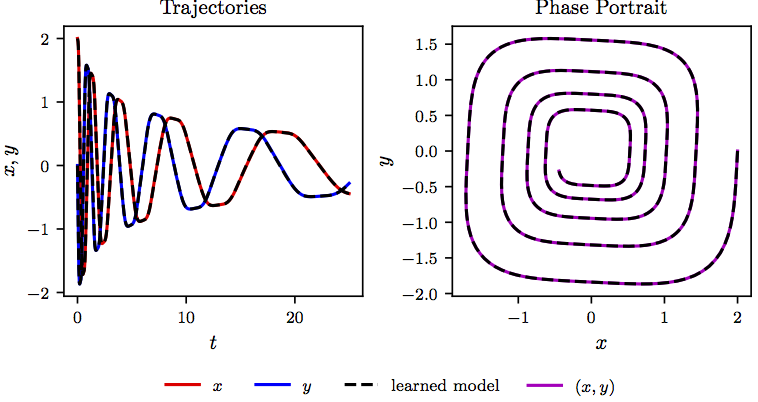
\[\begin{array}{l} \dot{x} = -0.1\ x^3 + 2.0\ y^3,\\ \dot{y} = -2.0\ x^3 - 0.1\ y^3. \end{array}\]We use \([x_0\ y_0]^T = [2\ 0]^T\) as initial condition and collect data from \(t = 0\) to \(t = 25\) with a time-step size of \(\Delta t = 0.01\). The data are plotted in the following figure. We employ a neural network with one hidden layer and 256 neurons to represent the nonlinear dynamics. As for the multistep scheme, we use Adams-Moulton with \(M=1\) steps (i.e., the trapezoidal rule). Upon training the neural network, we solve the identified system using the same initial condition as the one above. The following figure provides a qualitative assessment of the accuracy in identifying the correct nonlinear dynamics. Specifically, by comparing the exact and predicted trajectories of the system, as well as the resulting phase portraits, we observe that the algorithm can correctly capture the dynamic evolution of the system.
Lorenz system
To explore the identification of chaotic dynamics evolving on a finite dimensional attractor, we consider the nonlinear Lorenz system
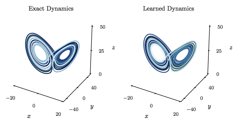
\[\begin{array}{l} \dot{x} = 10 (y - x),\\ \dot{y} = x (28 - z) - y,\\ \dot{z} = x y - (8/3) z. \end{array}\]We use \([x_0\ y_0\ z_0]^T = [-8\ 7\ 27]^T\) as initial condition and collect data from \(t = 0\) to \(t = 25\) with a time-step size of \(\Delta t = 0.01\). The data are plotted in the following figure. We employ a neural network with one hidden layer and 256 neurons to represent the nonlinear dynamics. As for the multistep scheme, we use Adams-Moulton with \(M=1\) steps (i.e., the trapezoidal rule). Upon training the neural network, we solve the identified system using the same initial condition as the one above. As depicted in the following figure, the learned system correctly captures the form of the attractor. The Lorenz system has a positive Lyapunov exponent, and small differences between the exact and learned models grow exponentially, even though the attractor remains intact.
Fluid flow behind a cylinder
In this example we collect data for the fluid flow past a cylinder at Reynolds number 100 using direct numerical simulations of the two dimensional Navier-Stokes equations (see the following figure).
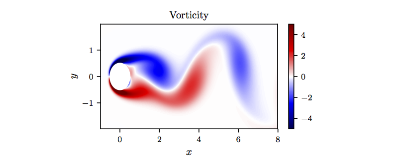
In particular, we simulate the Navier-Stokes equations describing the two-dimensional fluid flow past a circular cylinder at Reynolds number 100 using the Immersed Boundary Projection Method. This approach utilizes a multi-domain scheme with four nested domains, each successive grid being twice as large as the previous one. Length and time are non-dimensionalized so that the cylinder has unit diameter and the flow has unit velocity. Data is collected on the finest domain with dimensions \(9 \times 4\) at a grid resolution of \(449 \times 199\). The flow solver uses a 3rd-order Runge-Kutta integration scheme with a time step of \(t = 0.02\), which has been verified to yield well-resolved and converged flow fields. After simulations converge to steady periodic vortex shedding, flow snapshots are saved every \(\Delta t = 0.02\). We then reduce the dimension of the system by proper orthogonal decomposition (POD). The POD results in a hierarchy of orthonormal modes that, when truncated, capture most of the energy of the original system for the given rank truncation. The first two most energetic POD modes capture a significant portion of the energy; the steady-state vortex shedding is a limit cycle in these coordinates. An additional mode, called the shift mode, is included to capture the transient dynamics connecting the unstable steady state with the mean of the limit cycle. The resulting POD coefficients are depicted in the following figure.
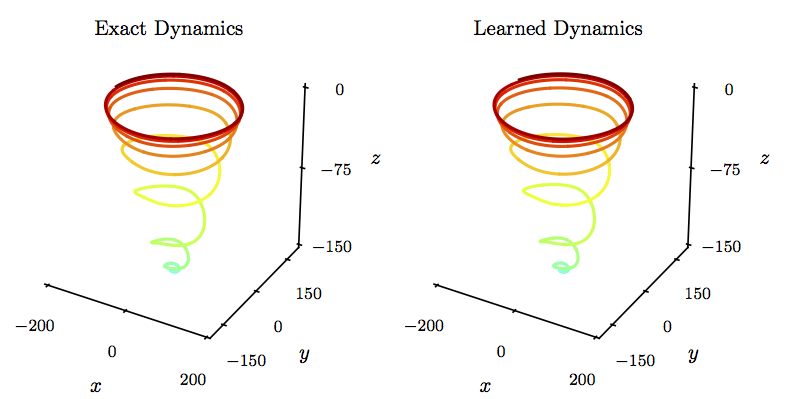
We employ a neural network with one hidden layer and \(256\) neurons to represent the nonlinear dynamics shown in the above figure. As for the linear multistep scheme, we use Adams-Moulton with \(M=1\) steps (i.e., the trapezoidal rule). Upon training the neural network, we solve the identified system. As depicted in the above figure, the learned system correctly captures the form of the dynamics and accurately reproduces the phase portrait, including both the transient regime as well as the limit cycle attained once the flow dynamics converge to the well known Karman vortex street.
Hopf bifurcation
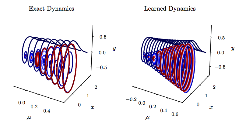
Many real-world systems depend on parameters and, when the parameters are varied, they may go through bifurcations. To illustrate the ability of our method to identify parameterized dynamics, let us consider the Hopf normal form
\[\begin{array}{l} \dot{x} = \mu x + y - x(x^2 + y^2),\\ \dot{y} = -x + \mu y - y(x^2 + y^2). \end{array}\]Our algorithm can be readily extended to encompass parameterized systems. In particular, the above system can be equivalently written as
\[\begin{array}{l} \dot{\mu} = 0,\\ \dot{x} = \mu x + y - x(x^2 + y^2),\\ \dot{y} = -x + \mu y - y(x^2 + y^2). \end{array}\]We collect data from the Hopf system for various initial conditions corresponding to different parameter values for \(\mu\). The data is depicted in the following figure. The identified parameterized dynamics is shown in the following figure for a set of parameter values different from the ones used during model training. The learned system correctly captures the transition from the fixed point for \(\mu < 0\) to the limit cycle for \(\mu>0\).
Glycolytic oscillator
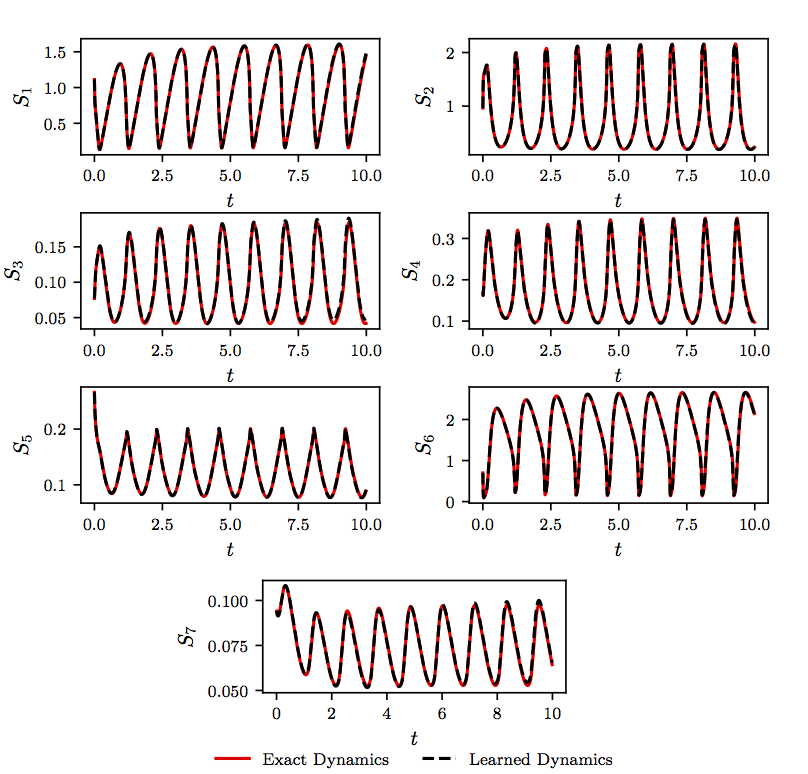
As an example of complicated nonlinear dynamics typical of biological systems, we simulate the glycolytic oscillator model. The model consists of ordinary differential equations for the concentrations of 7 biochemical species; i.e.,
\[\begin{array}{l} \frac{dS_1}{dt} = J_0 - \frac{k_1 S_1 S_6}{1 + (S_6/K_1)^q},\\ \frac{dS_2}{dt} = 2\frac{k_1 S_1 S_6}{1 + (S_6/K_1)^q} - k_2 S_2 (N - S_5) - k_6 S_2 S_5,\\ \frac{dS_3}{dt} = k_2 S_2 (N - S_5) - k_3 S_3 (N - S_6),\\ \frac{dS_4}{dt} = k_3 S_3 (A - S_6) - k_4 S_4 S_5 - \kappa (S_4 - S_7),\\ \frac{dS_5}{dt} = k_2 S_2 (N - S_5) - k_4 S_4 S_5 - k_6 S_2 S_5,\\ \frac{dS_6}{dt} = -2\frac{k_1 S_1 S_6}{1 + (S_6/K_1)^q} + 2 k_3 S_3 (A - S_6) - k_5 S_6,\\ \frac{dS_7}{dt} = \psi \kappa (S_4 - S_7) - k S_7. \end{array}\]As shown in the following figure, data from a simulation of this equation are collected from \(t = 0\) to \(t = 10\) with a time-step size of \(\Delta t = 0.01\). We employ a neural network with one hidden layer and \(256\) neurons to represent the nonlinear dynamics. As for the multi-step scheme, we use Adams-Moulton with \(M=1\) steps (i.e., the trapezoidal rule). Upon training the neural network, we solve the identified system using the same initial condition as the ones used for the exact system. As depicted in the following figure, the learned system correctly captures the form of the dynamics.
Conclusion
We have presented a machine learning approach for extracting nonlinear dynamical systems from time-series data. The proposed algorithm leverages the structure of well studied multi-step time-stepping schemes such as Adams-Bashforth, Adams Moulton, and BDF families, to construct efficient algorithms for learning dynamical systems using deep neural networks. Although state-of-the-art results are presented for a diverse collection of benchmark problems, there exist a series of open questions mandating further investigation. How could one handle a variable temporal gap \(\Delta{t}\), i.e., irregularly sampled data in time? How would common techniques such as batch normalization, drop out, and \(\mathcal{L}_1\)/\(\mathcal{L}_2\) regularization enhance the robustness of the proposed algorithm and mitigate the effects of over-fitting? How could one incorporate partial knowledge of the dynamical system in cases where certain interaction terms are already known? In terms of future work, interesting directions include the application of convolutional architectures for mitigating the complexity associated with very high-dimensional inputs.
Acknowledgements
This work received support by the DARPA EQUiPS grant N66001-15-2-4055 and the AFOSR grant FA9550-17-1-0013. All data and codes are publicly available on GitHub.
Citation
@article{raissi2018multistep,
  title={Multistep Neural Networks for Data-driven Discovery of Nonlinear Dynamical Systems},
  author={Raissi, Maziar and Perdikaris, Paris and Karniadakis, George Em},
  journal={arXiv preprint arXiv:1801.01236},
  year={2018}
}