Multi-fidelity Modeling
Design Optimization of an Ultrafast Marine Vehicle
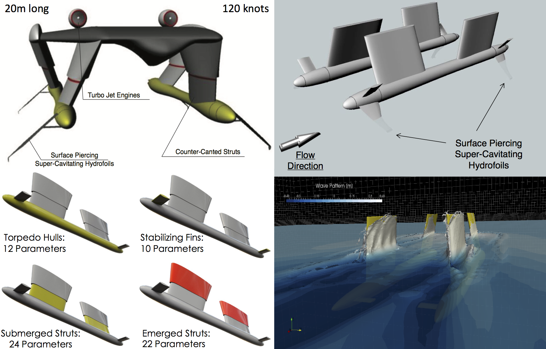
Multi-fidelity modeling enables the seamless fusion of information from a collection of heterogeneous sources of variable accuracy and cost (e.g., noisy experimental data, computer simulations, empirical models, etc.). By learning to exploit the cross-correlation structure between these sources, one can construct predictive surrogate models that can dramatically reduce the compute time to solution. The impact of multi-fidelity modeling has already been recognized in our project on shape optimization of super-cavitating hydrofoils. The application involves the design optimization of an ultrafast marine vehicle for special naval operations.

This problem inherits numerous and laborious challenges including the modeling of complex turbulent and multi-phase fluid flows, the solution of high-dimensional optimization problems, and the assessment of risk due to uncertainty in environmental and operational conditions. Here, the introduction of multi-fidelity modeling enables us to combine high-fidelity turbulent multi-phase flow simulations, experimental data, and simplified low-fidelity models (e.g., potential flow simulations), and efficiently tackle this large-scale optimization task that currently seems daunting to any other approach.
Deep Multi-fidelity Gaussian Processes
A simple way to explain the main idea of this work is to consider the following structure:
\[\begin{bmatrix} f_1(h) \\ f_2(h) \end{bmatrix} \sim \mathcal{GP}\left( \begin{bmatrix} 0 \\ 0 \end{bmatrix} , \begin{bmatrix} k_{1}(h,h') & \rho k_{1}(h,h') \\ \rho k_{1}(h,h') & \rho^2 k_{1}(h,h') + k_2(h,h') \end{bmatrix} \right),\]where
\[x \longmapsto h := h(x) \longmapsto \begin{bmatrix} f_1(h(x)) \\ f_2(h(x)) \end{bmatrix}.\]The high fidelity system is modeled by \(f_2(h(x))\) and the low fidelity one by \(f_1(h(x))\). We use \(\mathcal{GP}\) to denote a Gaussian Process. This approach can use any deterministic parametric data transformation \(h(x)\). However, we focus on multi-layer neural networks
\[h(x) := (h^L \circ \ldots \circ h^1) (x),\]where each layer of the network performs the transformation
\[h^\ell(z) = \sigma^\ell(w^\ell z + b^\ell),\]with \(\sigma^\ell\) being the transfer function, \(w^\ell\) the weights, and \(b^\ell\) the bias of the layer. We use \(\theta_h:= [w^1,b^1,\ldots,w^L,b^L]\) to denote the parameters of the neural network. Moreover, \(\theta_1\) and \(\theta_2\) denote the hyper-parameters of the covariance functions \(k_1\) and \(k_2\), respectively. The parameters of the model are therefore given by
\[\theta := [\rho,\theta_1,\theta_2,\theta_h].\]Prediction
The Deep Multi-fidelity Gaussian Process structure can be equivalently written in the following compact form of a multivariate Gaussian Process
\[\begin{bmatrix} f_1(h) \\ f_2(h) \end{bmatrix} \sim \mathcal{GP}\left( \begin{bmatrix} 0 \\ 0 \end{bmatrix} , \begin{bmatrix} k_{11}(h,h') & k_{12}(h,h') \\ k_{21}(h,h') & k_{22}(h,h') \end{bmatrix} \right)\]with \(k_{11} \equiv k_1, k_{12} \equiv k_{21} \equiv \rho k_1\), and \(k_{22} \equiv \rho^2 k_1 + k_2\). This can be used to obtain the predictive distribution
\[p\left(f_2(h(x_*))|x_*,\mathbf{x_1},\mathbf{f}_1,\mathbf{x_2},\mathbf{f}_2\right)\]of the surrogate model for the high fidelity system at a new test point \(x_*\). Note that the terms \(k_{12}(h(x),h(x'))\) and \(k_{21}(h(x),h(x'))\) model the correlation between the high-fidelity and the low-fidelity data and therefore are of paramount importance. The key role played by \(\rho\) is already well-known in the literature. Along the same lines one can easily observe the effectiveness of learning the transformation function $h(x)$ jointly from the low fidelity and high fidelity data.
We obtain the following joint density:
\[\begin{bmatrix} f_2(h(x_*)) \\ \mathbf{f}_1 \\ \mathbf{f}_2 \end{bmatrix} \sim \mathcal{N}\left( \begin{bmatrix} 0 \\ \mathbf{0} \\ \mathbf{0} \end{bmatrix}, \begin{bmatrix} k_{22}(h_*,h_*) & k_{21}(h_*,\mathbf{h}_1) & k_{22}(h_*,\mathbf{h}_2) \\ k_{12}(\mathbf{h}_1,h_*) & k_{11}(\mathbf{h}_1,\mathbf{h}_1) & k_{12}(\mathbf{h}_1,\mathbf{h}_2) \\ k_{22}(\mathbf{h}_2,h_*) & k_{21}(\mathbf{h}_2,\mathbf{h}_1) & k_{22}(\mathbf{h}_2,\mathbf{h}_2) \end{bmatrix} \right),\]where \(h_* = h(x_*)\), \(\mathbf{h}_1 = h(\mathbf{x}_1)\), and \(\mathbf{h}_2 = h(\mathbf{x}_2)\). From this, we conclude that
\[p\left(f_2(h(x_*))|x_*,\mathbf{x_1},\mathbf{f}_1,\mathbf{x_2},\mathbf{f}_2\right) = \mathcal{N}\left(K_* K^{-1} \mathbf{f}, k_{22}(h_*,h_*) - K_* K^{-1} K_*^T\right),\]where
\[\mathbf{f} := \begin{bmatrix} \mathbf{f}_1 \\ \mathbf{f}_2 \end{bmatrix},\] \[K_* := \begin{bmatrix} k_{21}(h_*,\mathbf{h}_1) & k_{22}(h_*,\mathbf{h}_2) \end{bmatrix},\] \[K := \begin{bmatrix} k_{11}(\mathbf{h}_1,\mathbf{h}_1) & k_{12}(\mathbf{h}_1,\mathbf{h}_2) \\ k_{21}(\mathbf{h}_2,\mathbf{h}_1) & k_{22}(\mathbf{h}_2,\mathbf{h}_2) \end{bmatrix}.\]Training
The negative log marginal likelihood \(\mathcal{L}(\theta) := -\log p\left( \mathbf{f} | \mathbf{x}\right)\) is given by \begin{eqnarray}\label{Likelihood} \mathcal{L}(\theta) = \frac12 \mathbf{f}^T K^{-1}\mathbf{f} + \frac12 \log \left| K \right| + \frac{n_1 + n_2}{2}\log 2\pi, \end{eqnarray} where
\[\mathbf{x} := \begin{bmatrix} \mathbf{x}_1 \\ \mathbf{x}_2 \end{bmatrix}.\]The negative log marginal likelihood along with its Gradient can be used to estimate the parameters \(\theta\).

Conclusions
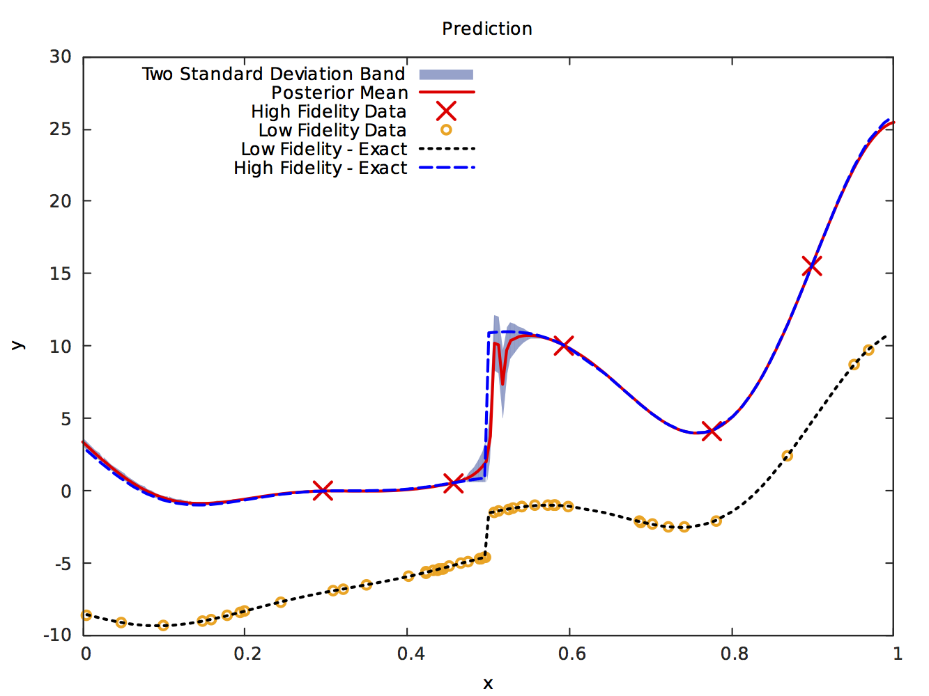
We devised a surrogate model that is capable of capturing general discontinuous correlation structures between the low- and high-fidelity data generating processes. The model’s efficiency in handling discontinuities was demonstrated using benchmark problems. Essentially, the discontinuity is captured by the neural network. The abundance of low-fidelity data allows us to train the network accurately. We therefore need very few observations of the high-fidelity data generating process.
Acknowledgments
This work was supported by the DARPA project on Scalable Framework for Hierarchical Design and Planning under Uncertainty with Application to Marine Vehicles (N66001-15-2-4055).
Citation
@article{raissi2016deep,
  title={Deep Multi-fidelity Gaussian Processes},
  author={Raissi, Maziar and Karniadakis, George},
  journal={arXiv preprint arXiv:1604.07484},
  year={2016}
}