Author

Abstract

This is a short tutorial on the following topics using Gaussian Processes: Gaussian Processes, Multi-fidelity Modeling, and Gaussian Processes for Differential Equations. The full code for this tutorial can be found here.

Gaussian Processes

A Gaussian process

$f(x) \sim \mathcal{GP}\left(0, k(x,x’;\theta)\right),$

is just a shorthand notation for saying

$\begin{bmatrix} f(x)\\ f(x’) \end{bmatrix} \sim \mathcal{N}\left(0, \begin{bmatrix} k(x,x;\theta) & k(x,x’;\theta)\\ k(x’,x;\theta) & k(x’,x’;\theta) \end{bmatrix} \right).$

A typical choice for the covariance function $k(x,x’;\theta)$ is the square exponential kernel

$k(x,x’;\theta) = \alpha^2 \exp\left(-\frac12 \sum_{d=1}^D \frac{(x_d - x_d’)^2}{\beta_d^2} \right),$

where $\theta = (\alpha, \beta)$ are the hyper-parameters.

Training

Given the training data $\{\mathbf{x}, \mathbf{y}\}$ , we make the assumption that

$\mathbf{y} = f(\mathbf{x}) + \mathbf{\epsilon}, \ \ \ \ \mathbf{\epsilon} \sim \mathcal{N}(\mathbf{0}, \sigma^2 \mathbf{I}).$

Consequently, we obtain

$\mathbf{y} \sim \mathcal{N}(\mathbf{0}, \mathbf{K}),$

where $\mathbf{K} = k(\mathbf{x}, \mathbf{x}; \theta) + \sigma^2 \mathbf{I}$ . The hyper-parameters $\theta$ and the noise variance parameter $\sigma^2$ can be trained by minimizing the resulting negative log marginal likelihood

$\mathcal{NLML}(\theta) = \frac12 \mathbf{y}^T \mathbf{K}^{-1} \mathbf{y} + \frac12 \log |\mathbf{K}| + \frac{N}{2} \log(2 \pi)$

Prediction

Prediction at a new test point $x^*$ can be made by first writing the joint distribution

$\begin{bmatrix} f(x^*)\\ \mathbf{y} \end{bmatrix} \sim \mathcal{N}\left(\mathbf{0}, \begin{bmatrix} k(x^*,x^*;\theta) & k(x^*,\mathbf{x};\theta)\\ k(\mathbf{x},x^*;\theta) & \mathbf{K} \end{bmatrix} \right).$

One can then use the resulting conditional distribution to make predictions

$f(x^*) | \mathbf{y} \sim \mathcal{N}\left(k(x^*,\mathbf{x})\mathbf{K}^{-1}\mathbf{y}, k(x^*,x^*) - k(x^*,\mathbf{x})\mathbf{K}^{-1}k(\mathbf{x},x^*) \right).$

Illustrative Example

The following figure depicts a Gaussian process fit to a synthetic dataset generated by random perturbations of a simple one dimensional function.

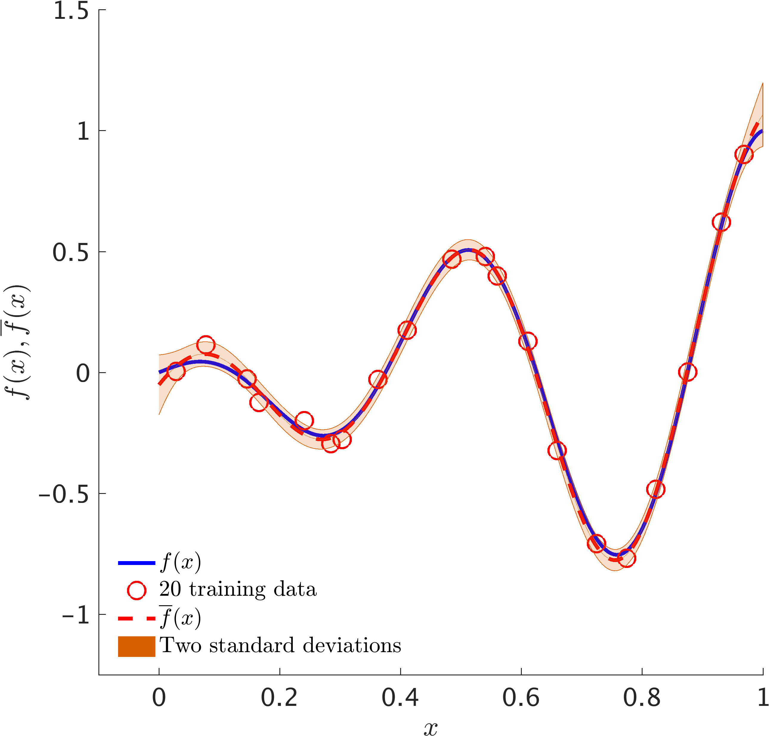
Illustrative Example: Training data along with the posterior distribution of the solution. The blue solid line represents the true data generating solution, while the dashed red line depicts the posterior mean. The shaded orange region specifies the two standard deviations band around the mean.

Multi-fidelity Gaussian Processes

Let us start by making the assumption that

$u_1(x) \sim \mathcal{GP}\left(0, k_1(x,x’;\theta_1)\right),$ $u_2(x) \sim \mathcal{GP}\left(0, k_2(x,x’;\theta_2)\right),$

are two independent Gaussian processes. We model the low fidelity function by $f_L(x) = u_1(x)$ and the hight-fidelity function by

$f_H(x) = \rho u_1(x) + u_2(x).$

This will result in the following multi-output Gaussian process

$\begin{bmatrix} f_L(x)\\ f_H(x) \end{bmatrix} \sim \mathcal{GP}\left(0, \begin{bmatrix} k_{LL}(x,x’;\theta_1) & K_{LH}(x,x’;\theta_1,\rho)\\ k_{HL}(x,x’;\theta_1,\rho) & K_{HH}(x,x’;\theta_1,\theta_2,\rho) \end{bmatrix}\right),$

where

$k_{LL}(x,x’;\theta_1) = k_1(x,x’;\theta_1),$ $k_{HL}(x,x’;\theta_1,\rho) = k_{LH}(x,x’;\theta_1,\rho) = \rho k_1(x,x’;\theta_1),$ $K_{HH}(x,x’;\theta_1,\theta_2,\rho) = \rho^2 k_1(x,x’;\theta_1) + k_2(x,x’;\theta_2),$

Training

Given the training data $\{\mathbf{x}_L, \mathbf{y}_L\}$ and $\{\mathbf{x}_H, \mathbf{y}_H\}$ , we make the assumption that

$\mathbf{y}_L = f_L(\mathbf{x}_L) + \mathbf{\epsilon}_L, \ \ \ \ \mathbf{\epsilon}_L \sim \mathcal{N}(\mathbf{0}, \sigma_L^2 \mathbf{I}),$

and

$\mathbf{y}_H = f_H(\mathbf{x}_H) + \mathbf{\epsilon}_H, \ \ \ \ \mathbf{\epsilon}_H \sim \mathcal{N}(\mathbf{0}, \sigma_H^2 \mathbf{I}).$

Consequently, we obtain

$\mathbf{y} \sim \mathcal{N}(\mathbf{0}, \mathbf{K}),$

where

$\mathbf{y} = \begin{bmatrix} \mathbf{y}_L \\ \mathbf{y}_H \end{bmatrix}$

and

$\mathbf{K} = \begin{bmatrix} k_{LL}(\mathbf{x}_L, \mathbf{x}_L; \theta_1) + \sigma_L^2 \mathbf{I} & k_{LH}(\mathbf{x}_L, \mathbf{x}_H; \theta_1, \rho)\\ k_{HL}(\mathbf{x}_H, \mathbf{x}_L; \theta_1) & k_{HH}(\mathbf{x}_H, \mathbf{x}_H; \theta_1, \theta_2, \rho) + \sigma_H^2 \mathbf{I}) \end{bmatrix}.$

The hyper-parameters $\theta_1, \theta_2, \rho$ and the noise variance parameters $\sigma_L^2, \sigma_H^2$ can be trained by minimizing the resulting negative log marginal likelihood

$\mathcal{NLML}(\theta_1, \theta_2, \rho) = \frac12 \mathbf{y}^T \mathbf{K}^{-1} \mathbf{y} + \frac12 \log |\mathbf{K}| + \frac{N}{2} \log(2 \pi)$

Prediction

Prediction at a new test point $x^*$ can be made by first writing the joint distribution

$\begin{bmatrix} f_H(x^*)\\ \mathbf{y} \end{bmatrix} \sim \mathcal{N}\left(\mathbf{0}, \begin{bmatrix} k_{HH}(x^*,x^*;\theta_1, \theta_2, \rho) & \mathbf{q}^T\\ \mathbf{q} & \mathbf{K} \end{bmatrix} \right),$

where

$\mathbf{q}^T = \begin{bmatrix} k_{HL}(x^*,\mathbf{x}_L; \theta_1, \rho) & k_{HH}(x^*,\mathbf{x}_H; \theta_1, \theta_2, \rho) \end{bmatrix}.$

One can then use the resulting conditional distribution to make predictions

$f_H(x^*) | \mathbf{y} \sim \mathcal{N}\left(\mathbf{q}^T \mathbf{K}^{-1} \mathbf{y}, k_{HH}(x^*,x^*) - \mathbf{q}^T\mathbf{K}^{-1}\mathbf{q} \right).$

Illustrative Example

The following figure depicts a multi-fidelity Gaussian process fit to a synthetic dataset generated by random perturbations of two simple one dimensional functions.

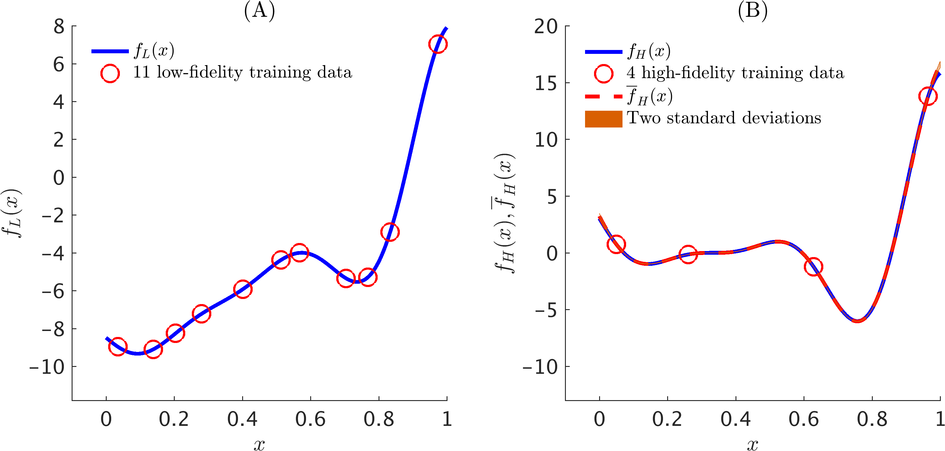
Illustrative Example: (A) Training low-fidelity data along with the true data generating low-fidelity function. (B) Training high-fidelity data along with the posterior distribution of the solution. The blue solid line represents the true data generating high-fidelity function, while the dashed red line depicts the posterior mean. The shaded orange region specifies the two standard deviations band around the mean.

Machine Learning of Linear Differential Equations using Gaussian Processes

A grand challenge with great opportunities facing researchers is to develop a coherent framework that enables them to blend differential equations with the vast data sets available in many fields of science and engineering. In particular, here we investigate governing equations of the form

where $u(x)$ is the unknown solution to a differential equation defined by the operator $\mathcal{L}_x^\phi$ , $f(x)$ is a black-box forcing term, and $x$ is a vector that can include space, time, or parameter coordinates. In other words, the relationship between $u(x)$ and $f(x)$ can be expressed as

$\mathcal{L}_x^\phi u(x) = f(x).$

Prior

The proposed data-driven algorithm for learning general parametric linear equations of the form presented above, employs Gaussian process priors that are tailored to the corresponding differential operators. Specifically, the algorithm starts by making the assumption that $u(x)$ is Gaussian process with mean $0$ and covariance function $k_{uu}(x,x';\theta)$ , i.e.,

$u(x) \sim \mathcal{GP}(0, k_{uu}(x,x';\theta)),$

where $\theta$ denotes the hyper-parameters of the kernel $k_{uu}$ . The key observation here is that any linear transformation of a Gaussian process such as differentiation and integration is still a Gaussian process. Consequently,

$\mathcal{L}_x^\phi u(x) = f(x) \sim \mathcal{GP}(0, k_{ff}(x,x';\theta,\phi)),$

with the following fundamental relationship between the kernels $k_{uu}$ and $k_{ff}$ ,

$k_{ff}(x,x';\theta,\phi) = \mathcal{L}_x^\phi \mathcal{L}^\phi_{x'} k_{uu}(x,x';\theta).$

Moreover, the covariance between $u(x)$ and $f(x')$ , and similarly the one between $f(x)$ and $u(x')$ , are given by $k_{uf}(x,x';\theta,\phi) = \mathcal{L}^\phi_{x'} k_{uu}(x,x';\theta)$ , and $k_{fu}(x,x';\theta,\phi) = \mathcal{L}^\phi_{x} k_{uu}(x,x';\theta)$ , respectively.

Training

The hyper-parameters $\theta$ and more importantly the parameters $\phi$ of the linear operator $\mathcal{L}_x^\phi$ can be trained by employing a Quasi-Newton optimizer L-BFGS to minimize the negative log marginal likelihood

$-\log p(\mathbf{y}| \phi, \theta, \sigma_{n_u}^2, \sigma_{n_f}^2) = \frac{1}{2}\log |\mathbf{K}| + \frac{1}{2} \mathbf{y}^{T}\mathbf{K}^{-1}\mathbf{y} + \frac{N}{2} \log 2\pi,$

where $\mathbf{y} = \begin{bmatrix} \mathbf{y}_u \\ \mathbf{y}_f \end{bmatrix}$ , $p(\mathbf{y} | \phi, \theta,\sigma_{n_u}^2,\sigma_{n_f}^2) = \mathcal{N}\left(\mathbf{0}, \mathbf{K}\right)$ , and $\mathbf{K}$ is given by

$\mathbf{K} = \begin{bmatrix} k_{uu}(\mathbf{X}_u,\mathbf{X}_u;\theta) + \sigma_{n_u}^2 \mathbf{I}_{n_u} & k_{uf}(\mathbf{X}_u,\mathbf{X}_f;\theta,\phi)\\ k_{fu}(\mathbf{X}_f,\mathbf{X}_u;\theta,\phi) & k_{ff}(\mathbf{X}_f,\mathbf{X}_f;\theta,\phi) + \sigma_{n_f}^2 \mathbf{I}_{n_f} \end{bmatrix}.$

Here, $\sigma_{n_u}^2$ and $\sigma_{n_f}^2$ are included to capture noise in the data and are also inferred from the data.

Prediction

Having trained the model, one can predict the values $u(x)$ and $f(x)$ at a new test point $x$ by writing the posterior distributions

$p(u(x) | \mathbf{y}) = \mathcal{N}\left(\overline{u}(x), s_u^2(x)\right),$ $p(f(x) | \mathbf{y}) = \mathcal{N}\left(\overline{f}(x), s_f^2(x)\right),$

with

$\overline{u}(x) = \mathbf{q}_u^T \mathbf{K}^{-1} \mathbf{y},\ s^2_u(x) = k_{uu}(x,x) - \mathbf{q}_u^T \mathbf{K}^{-1} \mathbf{q}_u,\nonumber\\ \overline{f}(x) = \mathbf{q}_f^T \mathbf{K}^{-1} \mathbf{y},\ s^2_f(x) = k_{ff}(x,x) - \mathbf{q}_f^T \mathbf{K}^{-1} \mathbf{q}_f,\nonumber$

where

$\mathbf{q}_u^T = \left[k_{uu}(x,\mathbf{X}_u) \ k_{uf}(x,\mathbf{X}_f)\right],$ $\mathbf{q}_f^T = \left[k_{fu}(x,\mathbf{X}_u)\ k_{ff}(x,\mathbf{X}_f)\right].$

Note that, for notational convenience, the dependence of kernels on hyper-parameters and other parameters is dropped. The posterior variances $s_u^2(x)$ and $s_f^2(x)$ can be used as good indicators of how confident one could be about predictions made based on the learned parameters $\phi$ .

Example: Fractional Equation

Consider the one dimensional fractional equation

$\mathcal{L}^{\alpha}_x u(x) = {}_{-\infty}D_x^\alpha u(x) - u(x) = f(x),$

where $\alpha = \sqrt{2}$ is the fractional order of the operator that is defined in the Riemann-Liouville sense. Fractional operators often arise in modeling anomalous diffusion processes and other non-local interactions. Their non-local behavior poses serious computational challenges as it involves costly convolution operations for resolving the underlying non-Markovian dynamics. However, the machine leaning approach pursued in this work bypasses the need for numerical discretization, hence, overcomes these computational bottlenecks, and can seamlessly handle all such linear cases without any modifications. The algorithm learns the parameter $\alpha$ to have value of $1.412104$ .

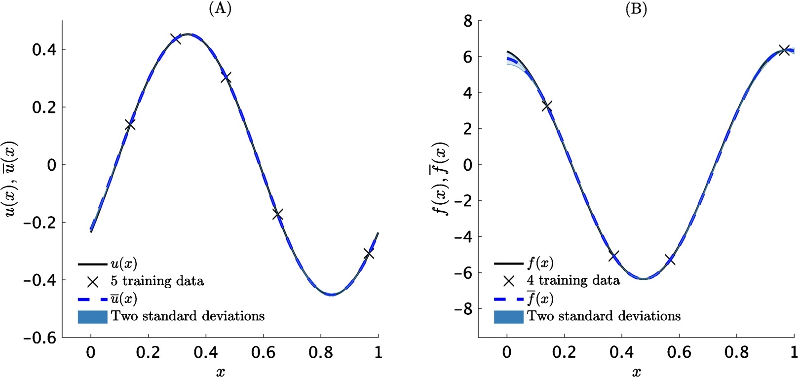
Fractional equation in 1D: (A) Exact left-hand-side function, training data, predictive mean, and two-standard-deviation band around the mean. (B) Exact right-hand-side function, training data, predictive mean, and two-standard-deviation band around the mean.

Example: Heat Equation

This example is chosen to highlight the ability of the proposed framework to handle time-dependent problems using only scattered space-time observations. To this end, consider the heat equation

$\mathcal{L}_{(t,x)}^\alpha u(t,x) := \frac{\partial}{\partial t} u(t,x) - \alpha \frac{\partial^2}{\partial x^2} u(t,x) = f(t,x).$

Here, $\alpha = 1$ . The algorithm learns the parameter $\alpha$ to have value of $0.999943$ .

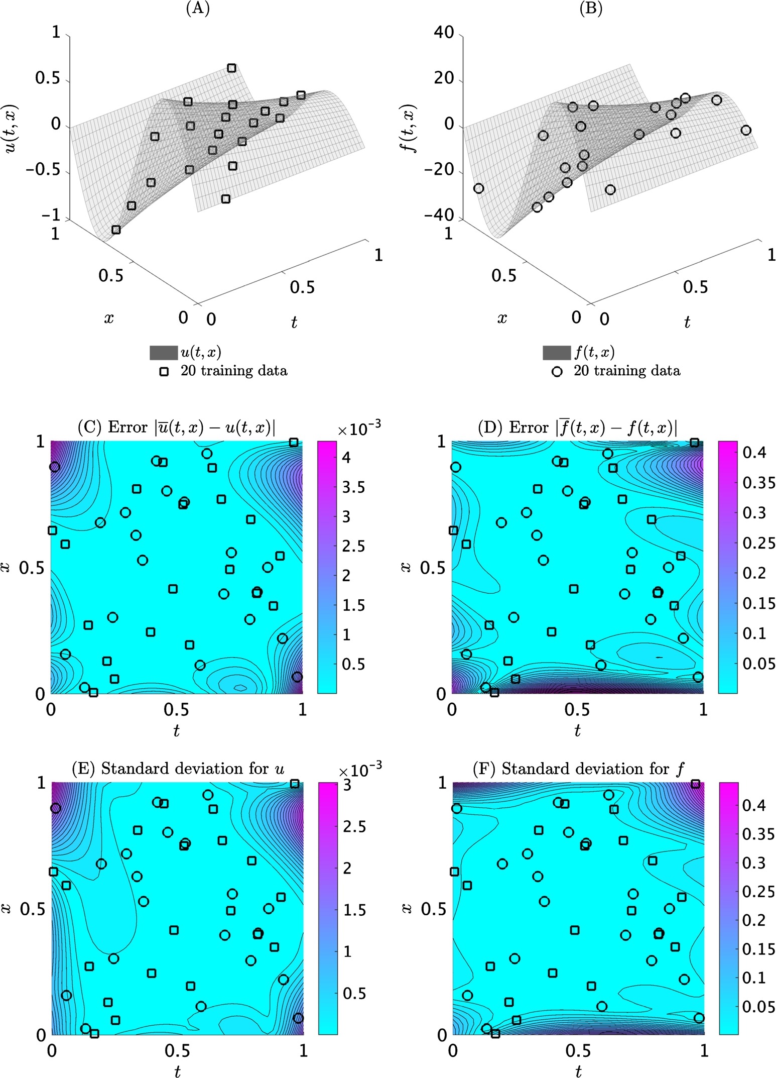
Heat equation: (A) Exact left-hand-side function and training data. (B) Exact right-hand-side function and training data. (C) Absolute point-wise error between the predictive mean and the exact function. The relative L2 error for the left-hand-side function is 1.25x10^-3. (D) Absolute point-wise error between the predictive mean and the exact function. The relative L2 error for the right-hand-side function is 4.17x10^-3. (E), (F) Standard deviations for the left- and rigt-hand-side functions, respectively.

Further Reading

For more information please refer to paper 1 and paper 2. The codes for these two papers are publicly available on GitHub.

All data and codes for this tutorial are publicly available on GitHub.

Citation

@article{raissi2016deep,
  title={Deep Multi-fidelity Gaussian Processes},
  author={Raissi, Maziar and Karniadakis, George},
  journal={arXiv preprint arXiv:1604.07484},
  year={2016}
}

@article{raissi2017inferring,
  title={Inferring solutions of differential equations using noisy multi-fidelity data},
  author={Raissi, Maziar and Perdikaris, Paris and Karniadakis, George Em},
  journal={Journal of Computational Physics},
  volume={335},
  pages={736--746},
  year={2017},
  publisher={Elsevier}
}

@article{RAISSI2017683,
  title = "Machine learning of linear differential equations using Gaussian processes",
  journal = "Journal of Computational Physics",
  volume = "348",
  pages = "683 - 693",
  year = "2017",
  issn = "0021-9991",
  doi = "https://doi.org/10.1016/j.jcp.2017.07.050",
  url = "http://www.sciencedirect.com/science/article/pii/S0021999117305582",
  author = "Maziar Raissi and Paris Perdikaris and George Em Karniadakis"
}

Gaussian Processes Tutorial

Tutorial on Gaussian Processes

Author

Abstract

Citation