Authors

Maziar Raissi, Paris Perdikaris, and George Em Karniadakis

Abstract

We introduce the concept of Numerical Gaussian Processes, which we define as Gaussian Processes with covariance functions resulting from temporal discretization of time-dependent partial differential equations. Numerical Gaussian processes, by construction, are designed to deal with cases where: (1) all we observe are noisy data on black-box initial conditions, and (2) we are interested in quantifying the uncertainty associated with such noisy data in our solutions to time-dependent partial differential equations. Our method circumvents the need for spatial discretization of the differential operators by proper placement of Gaussian process priors. This is an attempt to construct structured and data-efficient learning machines, which are explicitly informed by the underlying physics that possibly generated the observed data. The effectiveness of the proposed approach is demonstrated through several benchmark problems involving linear and nonlinear time-dependent operators. In all examples, we are able to recover accurate approximations of the latent solutions, and consistently propagate uncertainty, even in cases involving very long time integration.

Methodology

Problem Setup

Let us try to convey the main ideas of this work by considering the Burgers’ equation in one space dimension

$u_t + u u_x = \nu u_{xx},$

along with Dirichlet boundary conditions $u(t,-1)=u(t,1)=0,$ where $u(t,x)$ denotes the unknown solution and $\nu=0.01/\pi$ is a viscosity parameter. Let us assume that all we observe are noisy measurements $\{\mathbf{x}^0, \mathbf{u}^0\}$ of the black-box initial function $u(0,x)$ . Given such measurements, we would like to solve the Burgers’ equation while propagating through time the uncertainty associated with the noisy initial data.

Prior

Let us apply the backward Euler scheme to the Burgers’ equation. This can be written as

$u^{n} + \Delta t u^{n} \frac{d}{d x}u^{n} - \nu \Delta t \frac{d^2}{d x^2} u^n= u^{n-1}.$

Similar to the ideas presented here and here, we would like to place a Gaussian process prior on $u^n$ . However, the nonlinear term $u^{n} \frac{d}{d x}u^{n}$ is causing problems simply because the product of two Gaussian processes is no longer Gaussian. Hence, we will approximate the nonlinear term with $\mu^{n-1}\frac{d}{d x} u^{n}$ , where $\mu^{n-1}$ is the posterior mean of the previous time step. Therefore, the backward Euler scheme can be approximated by

$u^{n} + \Delta t \mu^{n-1} \frac{d}{d x}u^{n} - \nu \Delta t \frac{d^2}{d x^2} u^n = u^{n-1}.$

Let us make the prior assumption that

$u^{n}(x) \sim \mathcal{GP}(0, k(x,x';\theta)),$

is a Gaussian process with $\theta = \left(\sigma^{2}_0,\sigma^{2}\right)$ denoting the hyper-parameters of the kernel $k$ . This enables us to obtain the following Numerical Gaussian Process

$\begin{bmatrix} u^n\\ u^{n-1} \end{bmatrix} \sim \mathcal{GP}\left(0,\begin{bmatrix} k^{n,n}_{u,u} & k^{n,n-1}_{u,u}\\ k^{n-1,n}_{u,u} & k^{n-1,n-1}_{u,u} \end{bmatrix}\right).$

Training

The hyper-parameters $\theta$ and the noise parameters $\sigma_{n}^2, \sigma_{n-1}^2$ can be trained by employing the Negative Log Marginal Likelihood resulting from

$\begin{bmatrix} \mathbf{u}^{n}_b \\ \mathbf{u}^{n-1} \end{bmatrix} \sim \mathcal{N}\left(0,\mathbf{K}\right),$

where $\{\mathbf{x}^{n}_b, \mathbf{u}^{n}_b\}$ are the (noisy) data on the boundary and $\{\mathbf{x}^{n-1}, \mathbf{u}^{n-1}\}$ are artificially generated data to be explained later. Here,

$\mathbf{K} = \begin{bmatrix} k^{n,n}_{u,u}(\mathbf{x}_b^n, \mathbf{x}_b^n;\theta) + \sigma_{n}^2 \mathbf{I} & k^{n,n-1}_{u,u}(\mathbf{x}_b^n, \mathbf{x}^{n-1};\theta)\\ k^{n-1,n}_{u,u}(\mathbf{x}^{n-1}, \mathbf{x}_b^n;\theta) & k^{n,n-1}_{u,u}(\mathbf{x}^{n-1}, \mathbf{x}^{n-1};\theta) + \sigma_{n-1}^2 \mathbf{I} \end{bmatrix}$

Prediction & Propagating Uncertainty

In order to predict $u^{n}(x^{n})$ at a new test point $x^{n}$ , we use the following conditional distribution

$u^{n}(x^{n})\ |\ \mathbf{u}^{n}_b \sim \mathcal{N}\left(\mu^{n}(x^{n}), \Sigma^{n,n}(x^{n},x^{n})\right),$

where

$\mu^{n}(x^{n}) = \mathbf{q}^T \mathbf{K}^{-1}\begin{bmatrix} \mathbf{u}^{n}_b \\ \mathbf{\mu}^{n-1} \end{bmatrix},$

and

$\Sigma^{n,n}(x^{n},x^{n}) = k^{n,n}_{u,u}(x^{n},x^{n}) - \mathbf{q}^T\mathbf{K}^{-1}\mathbf{q} + \mathbf{q}^T\mathbf{K}^{-1} \begin{bmatrix} 0 & 0 \\ 0 & \mathbf{\Sigma}^{n-1,n-1} \end{bmatrix} \mathbf{K}^{-1}\mathbf{q}.$

Here, $\mathbf{q}^T = \left[k^{n,n}_{u,u}(x^n, \mathbf{x}_b^n)\ \ k^{n,n-1}_{u,u}(x^n, \mathbf{x}^{n-1})\right]$ .

Artificial data

Now, one can use the resulting posterior distribution to obtain the artificially generated data $\{\mathbf{x}^{n},\mathbf{u}^{n}\}$ for the next time step with

$\mathbf{u}^{n} \sim \mathcal{N}\left(\mathbf{\mu}^{n}, \mathbf{\Sigma}^{n,n} \right).$

Here, $\mathbf{\mu}^{n} = \mu^{n}(\mathbf{x}^{n})$ and $\mathbf{\Sigma}^{n,n} = \Sigma^{n,n}(\mathbf{x}^{n},\mathbf{x}^{n})$ .

Results

The code for this example can be found here and the corresponding movie is here.

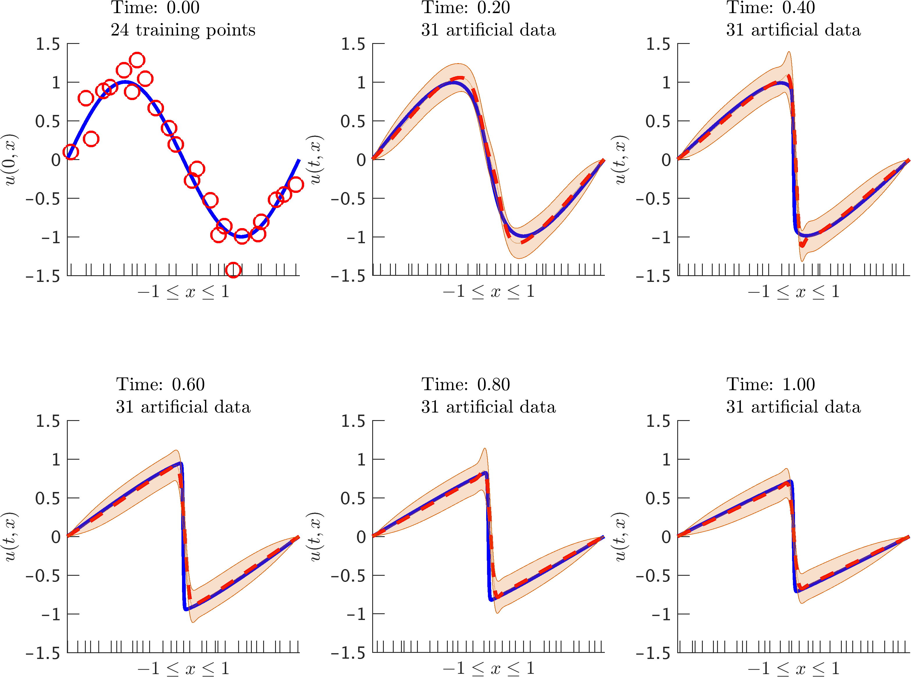
Burgers’ equation: Initial data along with the posterior distribution of the solution at different time snapshots. The blue solid line represents the true data generating solution, while the dashed red line depicts the posterior mean. The shaded orange region illustrates the two standard deviations band around the mean. We are employing the backward Euler scheme with time step size 0.01. At each time step we generate 31 artificial data points randomly located in the interval according to a uniform distribution. These locations are highlighted by the ticks along the horizontal axis.

Higher Order Time Stepping

Let us consider linear partial differential equations of the form

$u_t = \mathcal{L}_x u,$

where $\mathcal{L}_x$ is a linear operator and $u(t,x)$ denotes the latent solution.

Linear Multi-step Methods

As a representative member of the class of linear multi-step methods, let us consider the trapezoidal time-stepping scheme

$u^{n} - \frac12 \Delta t \mathcal{L}_x u^{n} = u^{n-1} + \frac12 \Delta t \mathcal{L}_x u^{n-1}.$

The trapezoidal time-stepping scheme can be equivalently written as

$u^{n} - \frac12 \Delta t \mathcal{L}_x u^{n} =: u^{n-1/2} := u^{n-1} + \frac12 \Delta t \mathcal{L}_x u^{n-1}$

By assuming $u^{n-1/2}(x) \sim \mathcal{GP}(0,k(x,x';\theta)),$ we can capture the entire structure of the trapezoidal rule in the resulting joint distribution of $u^n$ and $u^{n-1}$ .

Runge-Kutta Methods

The trapezoidal time-stepping scheme can be equivalently written as a representative member of the class of Runge-Kutta methods

$u^{n} = u^{n-1} + \Delta t \mathcal{L}_x u^{n-1/2},$ $u^{n-1/2} = u^{n-1} + \frac12 \Delta t \mathcal{L}_x u^{n-1/2}.$

Rearanging the terms we obtain

$u^{n-1}_2 := u^{n-1} = u^{n} - \Delta t \mathcal{L}_x u^{n-1/2},$ $u^{n-1}_1 := u^{n-1} = u^{n-1/2} - \frac12 \Delta t \mathcal{L}_x u^{n-1/2}.$

By assuming

$u^{n}(x) \sim \mathcal{GP}(0,k^{n,n}(x,x';\theta_n)),$ $u^{n-1/2}(x) \sim \mathcal{GP}(0,k^{n-1/2,n-1/2}(x,x';\theta_{n-1/2})),$

we can capture the entire structure of the trapezoidal rule in the resulting joint distribution of $u^n$ , $u^{n-1/2}$ , $u^{n-1}_2$ , and $u^{n-1}_1$ . Here, $u^{n-1}_2 = u^{n-1}_1 = u^{n-1}.$

Wave Equation

The code for this example can be found here and the corresponding movie is here.

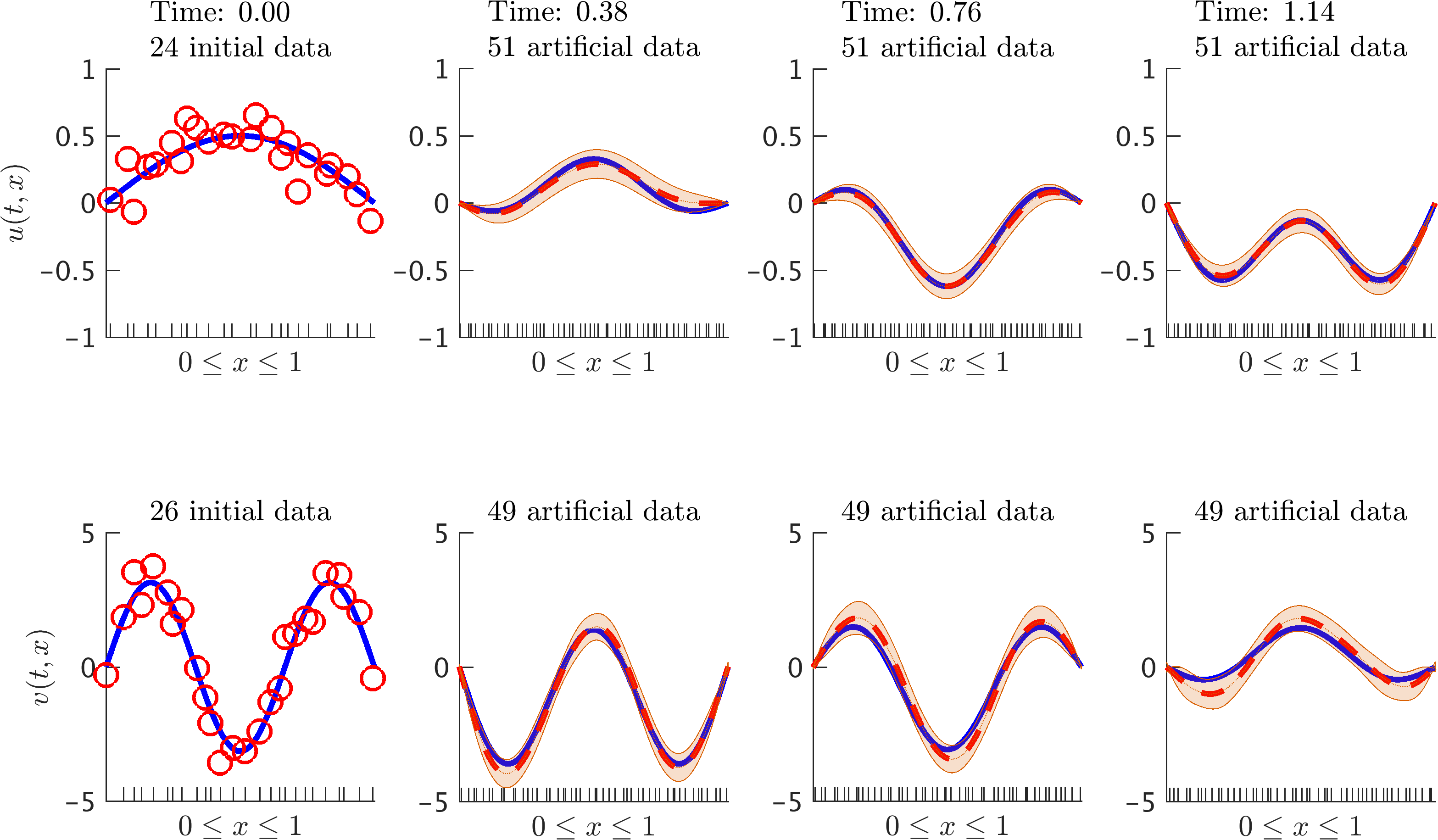
Wave equation: Initial data along with the posterior distribution of the solution at different time snapshots. Here, v denotes the time derivative of u. The blue solid line represents the true data generating solution, while the dashed red line depicts the posterior mean. The shaded orange region illustrates the two standard deviations band around the mean. At each time step we generate 51 artificial data points for u and 49 for v, all randomly located in the interval according to a uniform distribution. These locations are highlighted by the ticks along the horizontal axis. We are employing the trapezoidal scheme with time step size 0.01.

Advection Equation

The code for this example can be found here and the corresponding movie is here.

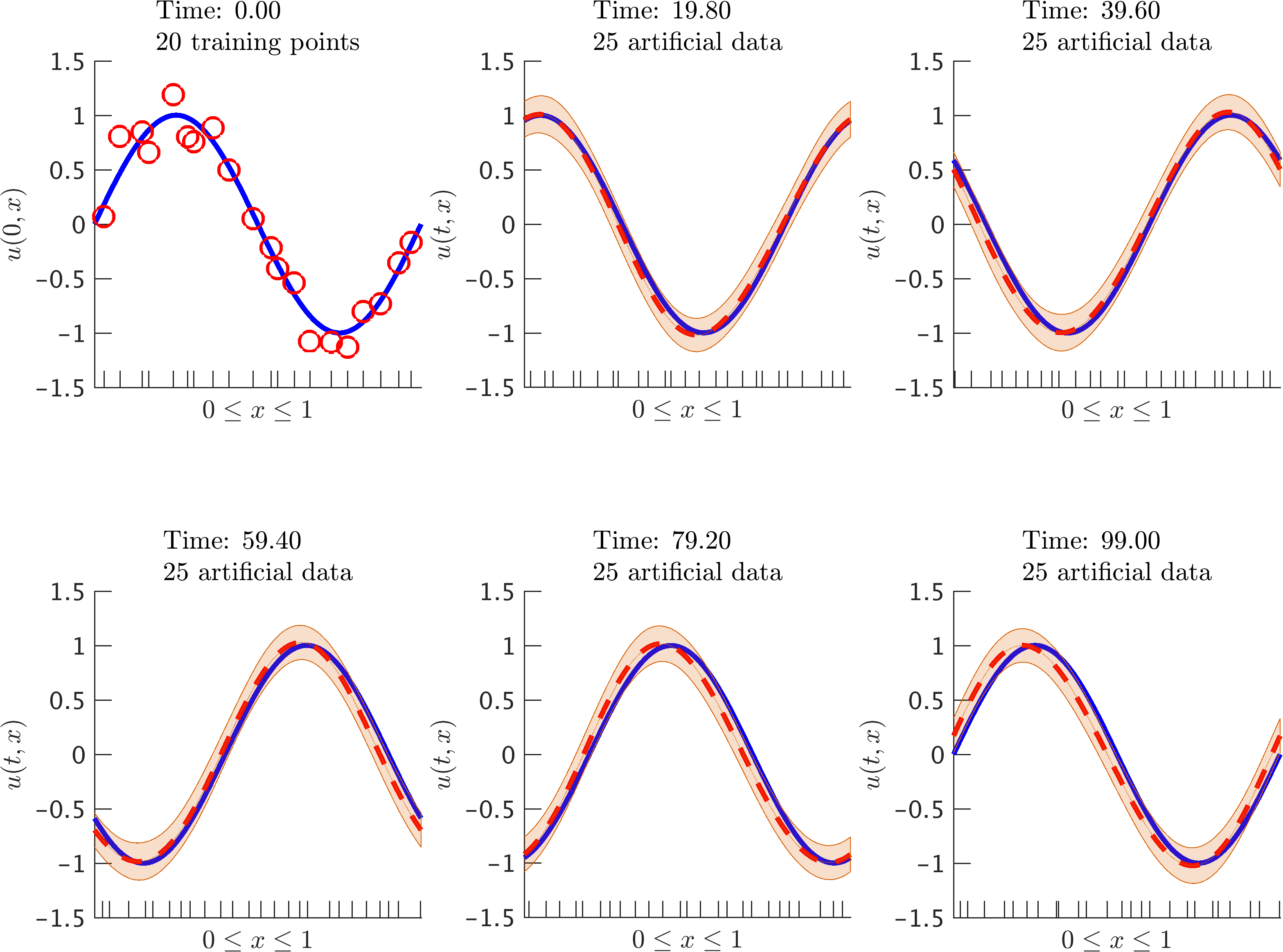
Advection equation: Initial data along with the posterior distribution of the solution at different time snapshots. The blue solid line represents the true data generating solution, while the dashed red line depicts the posterior mean. The shaded orange region illustrates the two standard deviations band around the mean. At each time step we generate 25 artificial data points randomly located in the interval according to a uniform distribution. These locations are highlighted by the ticks along the horizontal axis. We are employing the Gauss-Legendre time-stepping quadrature rule with time step size 0.1. It is worth highlighting that we are running the time stepping scheme for a very long time and with a relatively large time step size.

Heat Equation

The code for this example can be found here and the corresponding movie is here.

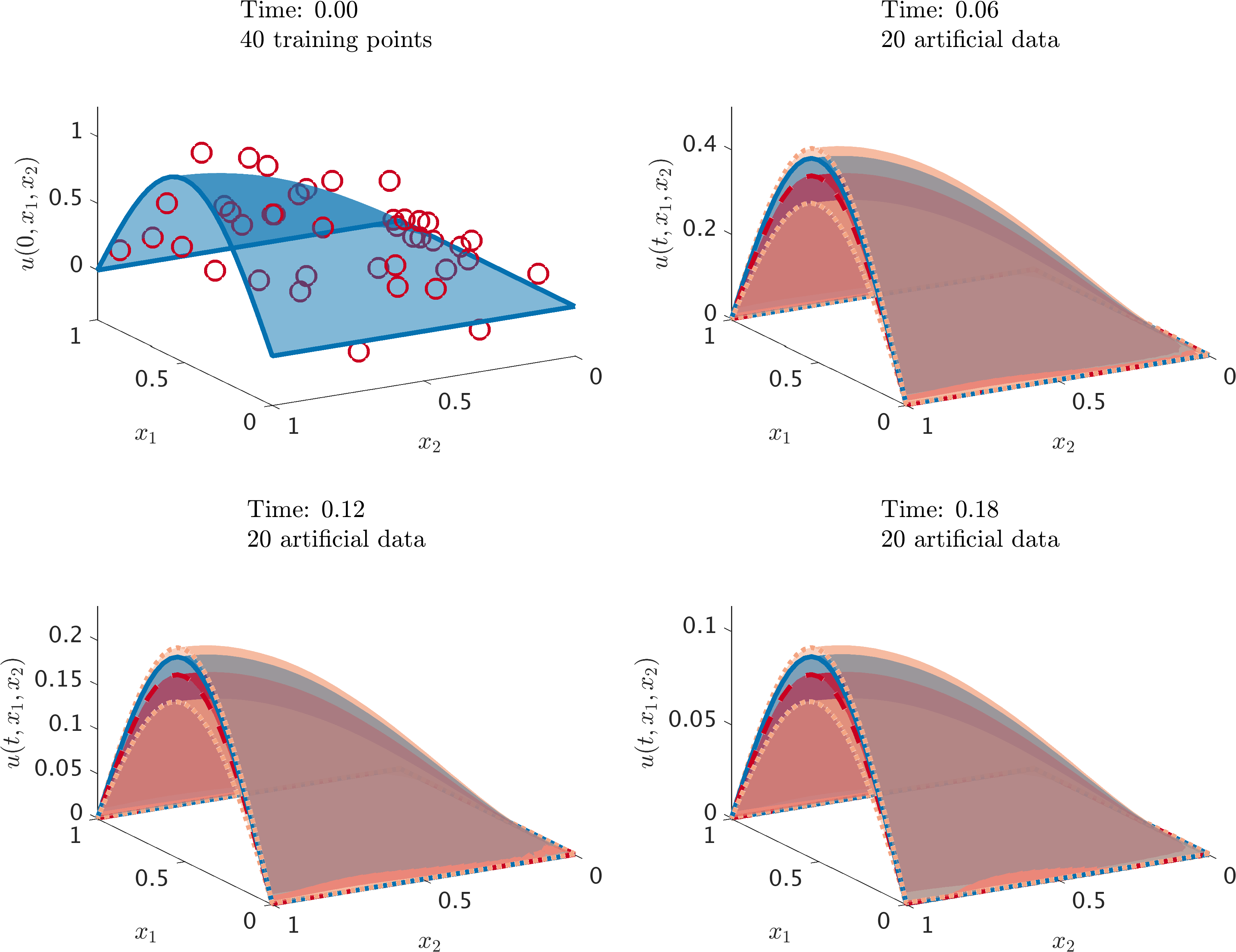
Heat equation: Initial data along with the posterior distribution of the solution at different time snapshots. The blue surface with solid lines represents the true data generating solution, while the red surface with dashed lines depicts the posterior mean. The two standard deviations band around the mean is depicted using the orange surface with dotted boundary. We are employing the trapezoidal rule with time step size 0.01. At each time step we generate 20 artificial data points randomly located in the domain according to a uniform distribution. We employ three noiseless data-points per boundary.

Conclusion

We have presented a novel machine learning framework for encoding physical laws described by partial differential equations into Gaussian process priors for nonparametric Bayesian regression. The proposed algorithms can be used to infer solutions to time-dependent and nonlinear partial differential equations, and effectively quantify and propagate uncertainty due to noisy initial or boundary data. Moreover, to the best of our knowledge, this is the first attempt to construct structured learning machines which are explicitly informed by the underlying physics that possibly generated the observed data. Exploiting this structure is critical for constructing data-efficient learning algorithms that can effectively distill information in the data-scarce scenarios appearing routinely when we study complex physical systems.

Acknowledgements

This work received support by the DARPA EQUiPS grant N66001-15-2-4055 and the AFOSR grant FA9550-17-1-0013. All data and codes are publicly available on GitHub.

Citation

@article{raissi2018numerical,
  title={Numerical Gaussian Processes for Time-Dependent and Nonlinear Partial Differential Equations},
  author={Raissi, Maziar and Perdikaris, Paris and Karniadakis, George Em},
  journal={SIAM Journal on Scientific Computing},
  volume={40},
  number={1},
  pages={A172--A198},
  year={2018},
  publisher={SIAM}
}

@article{raissi2017numerical,
  title={Numerical Gaussian Processes for Time-dependent and Non-linear Partial Differential Equations},
  author={Raissi, Maziar and Perdikaris, Paris and Karniadakis, George Em},
  journal={arXiv preprint arXiv:1703.10230},
  year={2017}
}

Numerical Gaussian Processes

Data-driven Solutions of Time-dependent and Non-linear Partial Differential Equations

Authors

Abstract

Citation